1. Introduction
Employee churn — the phenomenon of employees leaving an organization — is a critical challenge for businesses worldwide. High churn rates can disrupt operations, increase recruitment costs, and lower overall productivity. As organizations strive to retain top talent, predicting employee churn becomes a vital strategy.
Machine learning offers a data-driven approach to tackle this challenge. By analyzing employee-related data, we can identify patterns and key indicators associated with churn, enabling organizations to take proactive measures. This project demonstrates the power of machine learning in predicting employee churn, culminating in the development of an interactive application using Streamlit. The app provides two functionalities: single predictions based on user input and batch predictions using uploaded data files. This combination of machine learning and user-friendly deployment illustrates a practical and impactful solution for employee retention efforts.
2. Dataset Overview
The dataset used in this project, HR_comma_sep.csv, contains detailed information about employees, including their performance metrics, work history, and personal attributes. Below are the key features included in the dataset:
satisfaction_level: Employee satisfaction level (scaled between 0 and 1).
last_evaluation: Employee’s last performance evaluation score (scaled between 0 and 1).
number_project: Number of projects assigned to the employee.
average_monthly_hours: Average number of hours worked per month.
time_spend_company: Number of years spent at the company.
Work_accident: Binary indicator of whether the employee had a work-related accident (0 or 1).
promotion_last_5years: Binary indicator of whether the employee was promoted in the last five years (0 or 1).
department: Department the employee belongs to (e.g., sales, technical, support).
salary: Employee salary category (low, medium, high).
left: Target variable indicating whether the employee left the organization (1) or stayed (0).
This dataset provides a comprehensive view of factors that may contribute to an employee’s decision to leave or stay, making it a robust foundation for churn prediction.
3. Exploratory Data Analysis (EDA)
EDA provides insights into the structure and distribution of the dataset, helping identify patterns, trends, and potential issues. Below are key steps performed during EDA:
Dataset Summary
To understand the structure and basic statistics of the dataset:
import pandas as pd

data = pd.read_csv('HR_comma_sep.csv')

# Rename 'sales' column to 'department'
data.rename(columns={'sales': 'department'}, inplace=True)

# Display dataset information
data.info()

# Display summary statistics
print(data.describe())
<class 'pandas.core.frame.DataFrame'>
RangeIndex: 14999 entries, 0 to 14998
Data columns (total 10 columns):
 #   Column                 Non-Null Count  Dtype
---  ------                 --------------  -----
 0   satisfaction_level     14999 non-null  float64
 1   last_evaluation        14999 non-null  float64
 2   number_project         14999 non-null  int64
 3   average_montly_hours   14999 non-null  int64
 4   time_spend_company     14999 non-null  int64
 5   Work_accident          14999 non-null  int64
 6   left                   14999 non-null  int64
 7   promotion_last_5years  14999 non-null  int64
 8   department             14999 non-null  object
 9   salary                 14999 non-null  object
dtypes: float64(2), int64(6), object(2)
memory usage: 1.1+ MB
   satisfaction_level  last_evaluation  number_project  average_montly_hours  \
0                0.38             0.53               2                   157
1                0.80             0.86               5                   262
2                0.11             0.88               7                   272
3                0.72             0.87               5                   223
4                0.37             0.52               2                   159

   time_spend_company  Work_accident  left  promotion_last_5years department  \
0                   3              0     1                      0      sales
1                   6              0     1                      0      sales
2                   4              0     1                      0      sales
3                   5              0     1                      0      sales
4                   3              0     1                      0      sales

   salary
0     low
1  medium
2  medium
3     low
4     low
       satisfaction_level  last_evaluation  number_project  \
count        14999.000000     14999.000000    14999.000000
mean             0.612834         0.716102        3.803054
std              0.248631         0.171169        1.232592
min              0.090000         0.360000        2.000000
25%              0.440000         0.560000        3.000000
50%              0.640000         0.720000        4.000000
75%              0.820000         0.870000        5.000000
max              1.000000         1.000000        7.000000

       average_montly_hours  time_spend_company  Work_accident          left  \
count          14999.000000        14999.000000   14999.000000  14999.000000
mean             201.050337            3.498233       0.144610      0.238083
std               49.943099            1.460136       0.351719      0.425924
min               96.000000            2.000000       0.000000      0.000000
25%              156.000000            3.000000       0.000000      0.000000
50%              200.000000            3.000000       0.000000      0.000000
75%              245.000000            4.000000       0.000000      0.000000
max              310.000000           10.000000       1.000000      1.000000

       promotion_last_5years
count           14999.000000
mean                0.021268
std                 0.144281
min                 0.000000
25%                 0.000000
50%                 0.000000
75%                 0.000000
max                 1.000000
Analysis of Dataset Summary
- Dataset Structure:
The dataset contains 14,999 entries across 10 columns.
No missing values are present, as indicated by the non-null count for all columns.
Columns include numerical features (
satisfaction_level,last_evaluation, etc.) and categorical features (sales,salary).
2. Key Statistics:
Satisfaction Level:
Mean: 0.61, indicating moderate average satisfaction among employees.
Range: 0.09 to 1.00, showing varying levels of satisfaction.
Last Evaluation:
Mean: 0.72, suggesting overall high performance evaluations.
Range: 0.36 to 1.00, with most evaluations clustered around 0.72.
Number of Projects:
Mean: 3.8, with the majority of employees working on 3–5 projects.
Max: 7 projects, highlighting a subset of employees handling significantly higher workloads.
Average Monthly Hours:
Mean: 201 hours, with a wide range (96–310 hours).
High standard deviation (49.94), indicating variability in work intensity.
Time Spent at the Company:
Mean: 3.5 years, with most employees staying 3–4 years.
Maximum: 10 years, suggesting some long-tenured employees.
Work Accidents:
Mean: 0.14, showing that only about 14% of employees reported accidents.
Promotion in the Last 5 Years:
Mean: 0.02, indicating only 2% of employees received promotions, which might correlate with churn.
Churn (Left):
About 24% of employees (mean = 0.238) have left the organization.
3. Categorical Features:
Sales (Departments):
Represents department-level data, useful for understanding churn trends across roles.
Salary:
Categorical variable with levels (
low,medium,high), likely influencing churn behaviour.
Insights:
Churn Rate: With 24% churn, identifying the key factors contributing to employee departures is crucial.
Satisfaction Levels: Low satisfaction levels (min = 0.09) might indicate a strong correlation with churn.
Work Intensity: High variability in
average_monthly_hourssuggests some employees may be overburdened.Promotions: The low promotion rate (2%) could be a potential factor driving churn.
Departmental Trends: Further analysis of the
salesandsalaryfeatures is necessary to uncover trends influencing churn.
Visualizing Target Variable
Understanding the distribution of the target variable (left) helps gauge the proportion of employees who left versus those who stayed:
import seaborn as sns
import matplotlib.pyplot as plt

sns.countplot(data['left'])
plt.title('Employee Churn Distribution')
plt.xlabel('Left (1 = Yes, 0 = No)')
plt.ylabel('Count')
plt.show()

The plot indicates an imbalance in the dataset, with significantly more employees staying (0) than leaving (1). This imbalance highlights the need to handle the target variable during model training to avoid biased predictions, which PyCaret’s fix_imbalance=True can address.
Correlation Analysis
Examine the relationships between numerical features using a heatmap:
# Correlation heatmap
corr_matrix = data.corr()
sns.heatmap(corr_matrix, annot=True, cmap='coolwarm', fmt='.2f')
plt.title('Correlation Heatmap')
plt.show()

Key Correlations with Churn (
left):Negative Correlation:
satisfaction_level(-0.39): Lower satisfaction is strongly associated with higher churn.Positive Correlation:
time_spend_company(0.14): Employees with longer tenure are more likely to leave, potentially due to burnout or lack of growth opportunities.
Other Observations: Moderate correlation between
last_evaluationandaverage_monthly_hours(0.34) andnumber_project(0.35) suggests that highly evaluated employees tend to work more hours and handle more projects.
These insights guide feature importance and preprocessing steps, emphasizing the role of satisfaction and tenure in predicting churn.
Outlier Detection
Outliers can significantly impact model performance. To detect them, visualize key numerical features using boxplots:
# Outlier detection with boxplots
numerical_features = ['satisfaction_level', 'last_evaluation', 'number_project',
                      'average_montly_hours', 'time_spend_company']

for feature in numerical_features:
    plt.figure(figsize=(8, 4))
    sns.boxplot(x=data[feature])
    plt.title(f'Boxplot of {feature}')
    plt.show()
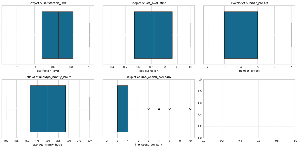
time_spend_company shows visible outliers for values greater than 5, indicating employees with unusually long tenures, while satisfaction_level, last_evaluation, number_project, and average_montly_hours show no significant outliers.
Since these high-tenure outliers may provide meaningful insights, we recommend relying on PyCaret’s built-in handling during the modelling process by enabling remove_outliers=True in the setup() function, instead of manually addressing them during preprocessing.
Analyzing Categorical Features
Explore categorical features like department and salary:
# Department-wise employee count
sns.countplot(y='department', hue='left', data=data)
plt.title('Employee Distribution by Department')
plt.xlabel('Count')
plt.ylabel('Department')
plt.show()
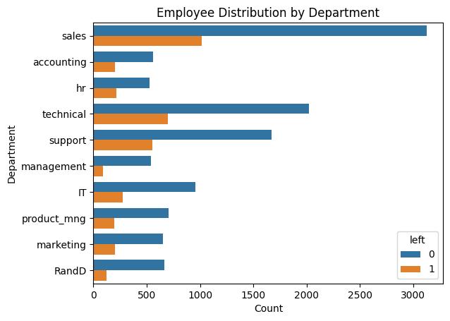
Analysis of the Employee Distribution by Department Plot:
- Churn Distribution Across Departments:
The sales department has the highest number of employees, followed by technical and support departments.
Churn (orange bars) is relatively higher in sales, technical, and support compared to other departments.
Departments like management and RandD show minimal churn.
2. Departmental Insights:
High churn in sales and technical roles could indicate job-related dissatisfaction or workload-related stress in these areas.
Lower churn in departments like management may suggest better job stability or satisfaction.
3. Implications for Retention Strategies:
Departments with higher churn (e.g., sales, technical) may require focused retention efforts, such as improving working conditions or providing incentives.
Further investigation into factors like satisfaction levels, workload, and salary in these departments could uncover actionable insights for reducing churn.
This analysis highlights the importance of tailoring retention strategies to department-specific needs.
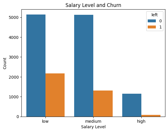
# Salary distribution and churn
sns.countplot(x='salary', hue='left', data=data)
plt.title('Salary Level and Churn')
plt.xlabel('Salary Level')
plt.ylabel('Count')
plt.show()
Analysis of the Employee Distribution by Department Plot:
- Churn Rate by Salary Level:
Employees with low salary levels have the highest churn rate, as indicated by a significant orange bar compared to those who stayed.
Employees with medium salaries show a moderate churn rate, lower than those with low salaries.
Employees with high salaries have an extremely low churn rate, with very few leaving the organization.
2. Insights:
Low salaries are a strong indicator of employee dissatisfaction and a key driver of churn.
Offering competitive salaries, especially for employees in the low and medium categories, could be an effective retention strategy.
3. Implication for Modeling:
- The
salaryfeature is likely to have significant predictive power in churn prediction and should be retained in the model.
This plot highlights the clear relationship between salary levels and churn, emphasizing the importance of salary as a retention factor.
4. Data Preprocessing
As we will use PyCaret — an AutoML tool — to handle much of the preprocessing and modelling, we only need to perform the essential tasks that PyCaret does not handle automatically:
Checking and Removing Duplicates
Remove any duplicate rows to ensure data quality:
# Remove duplicates if any
data.drop_duplicates(inplace=True)
Handling Outliers
While PyCaret can handle some outliers, it is often a good idea to manually review the data for extreme values:
# Example: Capping extreme values for 'average_monthly_hours'
data['average_monthly_hours'] = data['average_monthly_hours'].clip(lower=100, upper=300)
Data Type Verification
Ensure all columns have the correct data types:
# Verify and update data types if necessary
data['department'] = data['department'].astype('category')
data['salary'] = data['salary'].astype('category')
data['left'] = data['left'].astype('int')
These preprocessing steps ensure that the dataset is clean and ready for PyCaret to take over and handle scaling, encoding, and model training in the next stage.
5. Model Building and Evaluation
In this section, we use PyCaret — a robust AutoML tool — to build and evaluate multiple machine learning models efficiently. PyCaret automates preprocessing tasks such as scaling, encoding, and handling class imbalances, allowing us to focus on model selection and evaluation.
Setting Up PyCaret
Initialize the PyCaret environment with the preprocessed dataset:
from pycaret.classification import *

# Setting up the PyCaret environment
clf = setup(data=data, target='left',
            fix_imbalance=True,  # Handle class imbalance
            normalize=True)      # Scale numerical features
Comparing Models
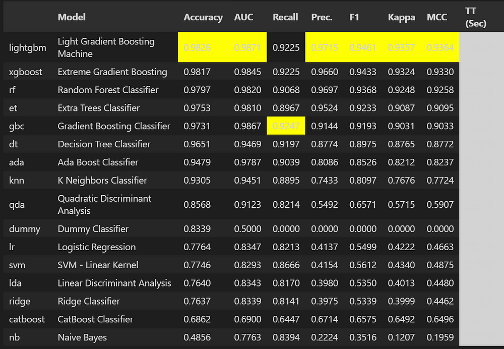
Use PyCaret’s compare_models function to train and evaluate multiple machine learning algorithms. This function ranks models based on their performance metrics:
# Compare models and select the best one
best_model = compare_models()
LightGBM is the best model for predicting employee churn, offering high accuracy and generalizability.
Fine-Tuning the Best Model
Once the best model is identified, fine-tune its hyperparameters to improve performance:
# Hyperparameter tuning
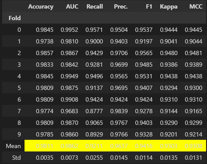
tuned_model = tune_model(best_model)
Fitting 10 folds for each of 10 candidates, totalling 100 fits
Original model was better than the tuned model, hence it will be returned. NOTE: The display metrics are for the tuned model (not the original one).
Evaluating the Final Model
Evaluate the tuned model using PyCaret’s built-in visualization tools:
# Evaluate the model
plot_model(tuned_model, plot='confusion_matrix')
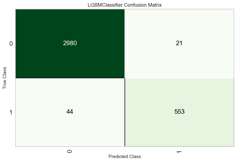
True Positives: 553 employees correctly identified as churners.
True Negatives: 2980 employees correctly identified as non-churners.
False Positives: Only 21, showing excellent precision.
False Negatives: 44, indicating some room for improvement in recall.
The model demonstrates strong stability across folds and excellent performance in both precision and recall, making it highly reliable for deployment.
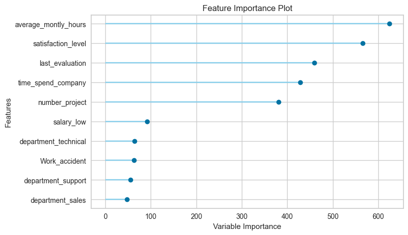
plot_model(tuned_model, plot='feature')
- Top Features:
average_montly_hoursis the most important feature, indicating that employees who work more hours are significantly linked to churn.satisfaction_levelis the second most influential factor, showing that lower satisfaction increases the likelihood of churn.
2. Moderately Important Features:
last_evaluationandtime_spend_companyplay notable roles, reflecting the impact of performance reviews and tenure on employee churn.number_projectalso has moderate importance, suggesting that workload affects retention.
3. Less Influential Features:
- Categorical features like
salary_lowand departmental indicators (e.g.,department_technical,department_support,department_sales) contribute less but still provide insights into churn patterns.
plot_model(tuned_model, plot='auc')
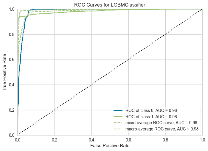
The ROC curve for the LGBMClassifier shows the following insights:
- AUC Scores:
Class 0 and Class 1 each have an AUC of 0.98, indicating excellent discrimination between the two classes.
The micro-average AUC (0.99) and macro-average AUC (0.98) confirm the model’s strong overall performance.
2. Performance at Different Thresholds:
The curve’s proximity to the top-left corner demonstrates high sensitivity (True Positive Rate) with minimal False Positives.
This is indicative of the model’s reliability in identifying both employees likely to stay and those likely to leave.
3. Balanced Performance:
- The nearly identical curves for each class suggest the model handles class imbalance effectively, likely aided by PyCaret’s
fix_imbalanceparameter during setup.
This curve highlights the LGBMClassifier’s robustness, making it a highly suitable choice for predicting employee churn.
Key Insights:
High working hours and low satisfaction are critical churn drivers.
Salary and departmental roles have limited but measurable effects on churn.
Finalizing the Model
Finalize the model to prepare it for deployment:
# Finalize the model
final_model = finalize_model(tuned_model)
The finalized model can now be used for predictions in the Streamlit application, ensuring a seamless workflow from training to deployment. PyCaret’s automation and visualization capabilities significantly simplify the machine learning process while ensuring high performance.
6. Developing and Deploying the Streamlit Application
The final step involves building and deploying an interactive Streamlit application. The application will allow users to input employee details or upload datasets to predict churn. Follow these steps:
Saving the Model
Before deploying, save the finalized model to a .pkl file for reuse in the Streamlit app:
import joblib

# Save the finalized model
joblib.dump(final_model, 'employee_churn_model.pkl')
['employee_churn_model.pkl']
Creating the Streamlit App (app.py)
Use Streamlit to create a user-friendly interface:
import streamlit as st
import pandas as pd
import joblib

# Load the saved model
model = joblib.load('employee_churn_model.pkl')
# Title and description
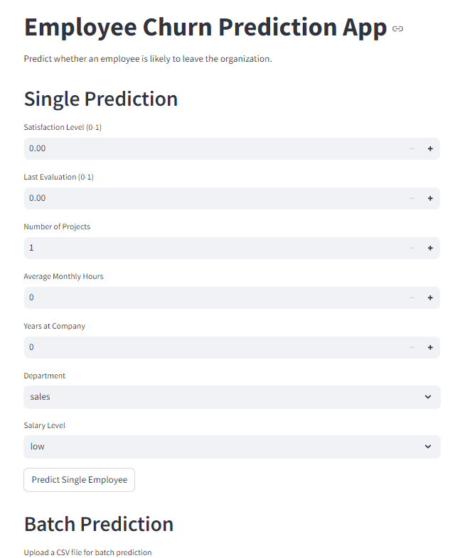
st.title('Employee Churn Prediction App')
st.write('Predict whether an employee is likely to leave the organization.')
# Single prediction input form
st.header('Single Prediction')
satisfaction_level = st.number_input('Satisfaction Level (0-1)', min_value=0.0, max_value=1.0, step=0.01)
last_evaluation = st.number_input('Last Evaluation (0-1)', min_value=0.0, max_value=1.0, step=0.01)
number_project = st.number_input('Number of Projects', min_value=1, step=1)
average_montly_hours = st.number_input('Average Monthly Hours', min_value=0, step=1)
time_spend_company = st.number_input('Years at Company', min_value=0, step=1)
department = st.selectbox('Department', ['sales', 'technical', 'support', 'management', 'IT', 'product_mng', 'marketing', 'RandD', 'hr', 'accounting'])
salary = st.selectbox('Salary Level', ['low', 'medium', 'high'])
# Predict button
if st.button('Predict Single Employee'):
    input_data = pd.DataFrame({
        'satisfaction_level': [satisfaction_level],
        'last_evaluation': [last_evaluation],
        'number_project': [number_project],
        'average_montly_hours': [average_montly_hours],
        'time_spend_company': [time_spend_company],
        'department': [department],
        'salary': [salary]
    })
    prediction = model.predict(input_data)[0]
    result = 'Employee is likely to leave.' if prediction == 1 else 'Employee is likely to stay.'
    st.write(result)
# Batch prediction
st.header('Batch Prediction')
uploaded_file = st.file_uploader('Upload a CSV file for batch prediction', type=['csv'])
if uploaded_file is not None:
    batch_data = pd.read_csv(uploaded_file)
    predictions = model.predict(batch_data)
    batch_data['Prediction'] = predictions
    st.write(batch_data)
    st.download_button('Download Predictions', batch_data.to_csv(index=False), file_name='predictions.csv')
Create a requirements.txt file
To ensure all dependencies are installed when deploying the app, create a requirements.txt file listing the necessary Python packages:
pandas
streamlit
scikit-learn
pycaret
joblib
Save this file in the same directory as the Streamlit app.
Running and Deploying the Application
To run the Streamlit app locally, use the command:
streamlit run app.py
To deploy the app online:
Push your repository to GitHub.
Use a platform like Streamlit Cloud.
Click the Deploy button in the top-right corner of the Streamlit Cloud interface to make the app publicly accessible.
This will launch the application in a web browser, allowing users to make single or batch predictions interactively. The result will look like this:
7. Conclusion
This project demonstrates the practical application of machine learning in predicting employee churn, providing organizations with actionable insights to reduce attrition rates. By leveraging PyCaret’s AutoML capabilities, we efficiently identified the best-performing model, Light Gradient Boosting Machine, which achieved excellent accuracy and recall.
The development of an interactive Streamlit app further enhances the project’s usability, enabling both single and batch predictions through a user-friendly interface. This integration bridges the gap between technical analysis and real-world application, empowering organizations to make data-driven decisions proactively.
Overall, this project highlights the value of combining machine learning and modern deployment tools to address critical business challenges effectively. Future work could focus on incorporating additional features, such as real-time data streaming and advanced visualization dashboards, to expand the scope and impact of the solution.
Appendices
Data source: https://www.kaggle.com/datasets/liujiaqi/hr-comma-sepcsv

