Predicting Ad Clicks with Logistic Regression: A Step-by-Step Guide Using Python

1. Introduction
Predicting user behavior has become an integral part of optimizing online advertising strategies. In this project, we explore how logistic regression can be used to predict whether a user will click on an advertisement based on their profile and activity. Using Python and its powerful libraries, we analyze a dataset of internet users to build and evaluate a classification model.
The dataset includes various features such as user age, income, daily internet usage, and time spent on the website. By leveraging exploratory data analysis (EDA) and scikit-learn’s logistic regression implementation, we aim to create a model that predicts ad clicks and provides insights into user behavior patterns. Whether you’re a beginner in machine learning or looking to enhance your project portfolio, this blog walks you through each step of the process.
2. Understanding the Dataset
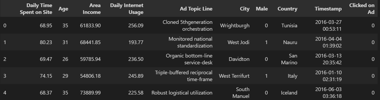
The dataset for this project, advertising.csv, contains 1,000 rows and 10 columns. It records the behavior and demographic attributes of internet users, as well as whether they clicked on an advertisement. Here's an overview of the key features:
Daily Time Spent on Site: Average time (in minutes) the user spends on the site daily.Age: Age of the user in years.Area Income: Average income of the user’s geographical region.Daily Internet Usage: Average time (in minutes) the user spends on the internet daily.Ad Topic Line: The headline text of the advertisement.City: The city where the user resides.Male: Indicates whether the user is male (1) or female (0).Country: The user’s country.Timestamp: The date and time of interaction with the ad.Clicked on Ad: The target variable, indicating whether the user clicked on the ad (1) or not (0).
3. Exploratory Data Analysis (EDA)
Exploratory Data Analysis (EDA) helps us uncover patterns, relationships, and insights from the dataset, forming the foundation for model building. In this section, we examine the dataset’s structure, distributions, and correlations using visualizations.
Data Summary
To start, we inspect the dataset’s structure and statistical properties. By examining data types, missing values, and summary statistics, we ensure that the dataset is ready for analysis.
# Load the dataset
import pandas as pd

ad_data = pd.read_csv("advertising.csv")
ad_data.head()
# Basic info
ad_data.info()
<class 'pandas.core.frame.DataFrame'>
RangeIndex: 1000 entries, 0 to 999
Data columns (total 10 columns):
Daily Time Spent on Site    1000 non-null float64
Age                         1000 non-null int64
Area Income                 1000 non-null float64
Daily Internet Usage        1000 non-null float64
Ad Topic Line               1000 non-null object
City                        1000 non-null object
Male                        1000 non-null int64
Country                     1000 non-null object
Timestamp                   1000 non-null object
Clicked on Ad               1000 non-null int64
dtypes: float64(3), int64(3), object(4)
memory usage: 78.2+ KB
Key observations:
The dataset contains 1,000 rows and 10 columns with no missing values.
Features like
Daily Time Spent on Site,Age, andArea Incomeshow meaningful numerical variation, ideal for modeling.The target variable,
Clicked on Ad, is binary (0or1).Visualizations to understand data distributions and relationships\
# Summary statistics
ad_data.describe()
Daily Time Spent on Site: Mean: 65 minutes, with a range from 32.6 to 91.43 minutes.Age: Mean: 36 years, ranging from 19 to 61 years. Besides, the majority of users are between 29 (25th percentile) and 42 (75th percentile).Area Income: Average income is $55,000, with values ranging from ~$14,000 to ~$79,000.Daily Internet Usage: Users spend an average of 180 minutes online, ranging from ~105 to ~270 minutes.Male: Binary column (0or1), with ~48% of users being male.Clicked on Ad: Target variable, equally distributed (50%1and 50%0).
These insights provide a strong foundation for visualizations and further analysis. Let me know if you’d like any additional interpretation!
Visualizing Feature Distributions
To better understand the distributions of the dataset’s features, we examine the histograms for multiple variables. This multi-variable analysis helps identify patterns and ensure the dataset is ready for modeling. Here’s the code used to generate these histograms:
# Visualizing distributions of all numeric features
ad_data[['Daily Time Spent on Site','Age','Area Income','Daily Internet Usage','Male','Clicked on Ad']].hist(figsize=(10,8))
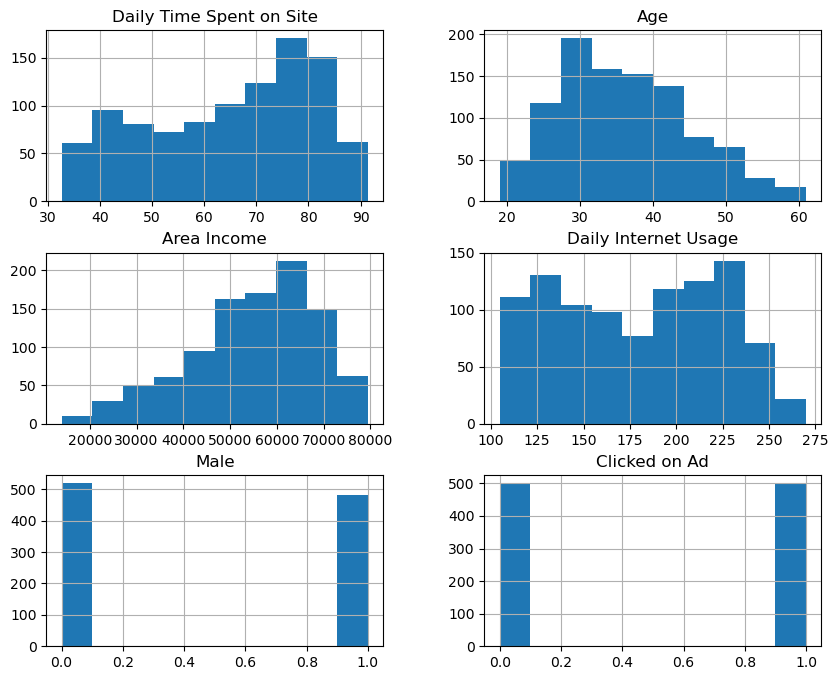
Interpretation:
Daily Time Spent on Site: Most users spend between 50 to 80 minutes daily on the site, with a slight skew toward higher usage.Age: The age distribution is approximately normal, with most users falling between 30 and 45 years.Area Income: The income distribution is also normal, centered around $55,000. A majority of users have incomes between $47,000 and $65,000.Daily Internet Usage: This feature shows a bimodal distribution, with clusters around 130 and 220 minutes of daily internet use.Male: TheMalecolumn is binary, showing a near-equal split between male (1) and female (0) users.Clicked on Ad: The target variable is balanced, with roughly 50% of users clicking on ads (1) and 50% not (0).
This concise representation of feature distributions lays the groundwork for understanding feature importance in predicting ad clicks.
Pair Plot for Feature Relationships
To analyze all numeric feature interactions simultaneously, we generate a pair plot, adding colour coding for the target variable, Clicked on Ad.
# Pairplot for all features
sns.pairplot(ad_data, hue='Clicked on Ad')
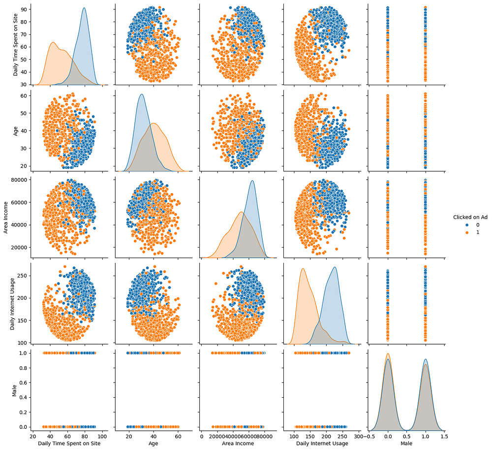
The pair plot provides insights into the relationships between numeric features and the target variable, Clicked on Ad:
Daily Time Spent on Site: Users who clicked on the ad (
1) tend to spend more time on the site, forming a clear separation from users who didn’t click (0).Age: Age shows a distinct pattern with ad clicks. Users in the middle age range (~30–45) are more likely to click on ads compared to younger or older users.
Area Income: There is no strong linear relationship between income and ad clicks, but higher incomes appear to have a slightly stronger association with not clicking the ad.
Daily Internet Usage: Users with lower daily internet usage are more likely to click on ads, while higher usage correlates with not clicking.
Male: The target variable (
Clicked on Ad) shows a relatively even split between genders, with no clear bias toward either male (1) or female (0).Overall Relationships:
Daily Time Spent on SiteandDaily Internet Usageshow distinct clusters based on the target variable.Features such as
AgeandArea Incomeexhibit moderate separability for ad clicks.
This pair plot highlights which features might be predictive of ad clicks and forms a basis for feature selection in modeling.
4. Data Preprocessing
Data preprocessing involves selecting relevant features and splitting the data into training and testing sets. Here’s how we prepared the dataset for modeling:
Feature Selection
Not all columns in the dataset contribute to predicting ad clicks. We select the following features:
Daily Time Spent on SiteAgeArea IncomeDaily Internet UsageMale
The target variable is Clicked on Ad. Irrelevant columns, such as Ad Topic Line, City, Country, and Timestamp, are dropped to focus on predictive features.
# Selecting features and target variable
X = ad_data[['Daily Time Spent on Site', 'Age', 'Area Income', 'Daily Internet Usage', 'Male']]
y = ad_data['Clicked on Ad']
Splitting the Data
To train and evaluate the model, the dataset is split into training and testing sets using an 80–20 split.
# Train-test split
from sklearn.model_selection import train_test_split

X_train, X_test, y_train, y_test = train_test_split(X, y, test_size=0.2, random_state=101)
Training Set: Used for building the logistic regression model.
Testing Set: Reserved for evaluating the model’s performance.
5. Building and Evaluating the Logistic Regression Model
With the preprocessed data, we now focus on building a logistic regression model to predict whether a user will click on an advertisement. Using scikit-learn, we train the model, make predictions, and evaluate its performance.
Training the Model
We start by importing the LogisticRegression class from scikit-learn and fitting the model on the training data.
from sklearn.linear_model import LogisticRegression

# Instantiate the logistic regression model
log_model = LogisticRegression()

# Train the model
log_model.fit(X_train, y_train)
The logistic regression model learns the relationships between the selected features and the target variable (Clicked on Ad).
Making Predictions
Once the model is trained, we use it to predict the outcomes for the test data.
# Make predictions on the test set
predictions = log_model.predict(X_test)
These predictions represent the model’s classification of whether each user in the test set clicked on the ad (1) or not (0).
Evaluating the Model
To evaluate the model, we use performance metrics such as the classification report and the confusion matrix. These metrics provide insights into the accuracy and effectiveness of the model.
from sklearn.metrics import classification_report, confusion_matrix

# Classification report
print(classification_report(y_test, predictions))

# Confusion matrix
print(confusion_matrix(y_test, predictions))
              precision    recall  f1-score   support

           0       0.91      0.94      0.93        89
           1       0.95      0.93      0.94       111

    accuracy                           0.94       200
   macro avg       0.93      0.94      0.93       200
weighted avg       0.94      0.94      0.94       200

[[ 84   5]
 [  8 103]]
The classification report and confusion matrix indicate that the logistic regression model performs well:
Accuracy: The model achieves a high overall accuracy of 94%, meaning it correctly predicts 94% of all test cases.
Class-Specific Performance:
Class 0 (Did not click):
Precision: 91% of predicted “no-click” cases are correct.
Recall: 94% of actual “no-click” cases are correctly identified.
F1-Score: 93%, showing a good balance between precision and recall.
Class 1 (Clicked):
Precision: 95% of predicted “click” cases are correct.
Recall: 93% of actual “click” cases are correctly identified.
F1-Score: 94%, reflecting high reliability.
3. Confusion Matrix:
True Positives (103): Correctly predicted ad clicks.
True Negatives (84): Correctly predicted non-clicks.
False Positives (5): Non-clicks are incorrectly predicted as clicks.
False Negatives (8): Clicks incorrectly predicted as non-clicks.
Overall, the model demonstrates strong precision and recall for both classes, with minimal misclassifications (5 false positives and 8 false negatives). This indicates a reliable and well-balanced model for predicting ad clicks.
6. Conclusion
In this project, we used logistic regression to predict whether a user would click on an advertisement based on features such as Age, Daily Time Spent on Site, Area Income, and Daily Internet Usage. The process involved data exploration, preprocessing, and model evaluation.
Key Takeaways:
Model Performance:
The logistic regression model achieved a high accuracy of 94%, with balanced precision and recall for both classes. This indicates that the model is effective in predicting user behavior.Feature Insights:
Users spending more time on the site were more likely to click on ads.
Middle-aged users showed a higher likelihood of clicking on advertisements compared to younger or older users.
Lower daily internet usage correlated with higher ad click rates.
3. Applications:
This model can be used by advertisers to target specific user segments more effectively, improving the efficiency of online marketing campaigns.
Next Steps:
To further improve the model, we could:
Experiment with additional features, such as text analysis of the ad topic line.
Explore advanced algorithms, such as decision trees or ensemble methods.
Perform hyperparameter tuning to optimize the logistic regression model.
This project demonstrates the practical use of logistic regression for classification tasks, providing valuable insights into user behavior and actionable predictions for advertisers.
Appendices
Data: https://www.kaggle.com/code/dipankarroydipu/advertising-data-analysis-logistic-regression


