
Photo by Jakub Żerdzicki on Unsplash
Enhanced Loan Status Prediction: Comparing Logistic Regression and SVM Models
1. Introduction
Predicting loan status is a critical task in the financial sector, helping lenders make informed decisions on loan approvals. Machine learning models offer powerful tools to streamline this process, providing accuracy and efficiency that traditional methods often lack.
In this project, we build a loan status prediction model using Logistic Regression and Support Vector Machines (SVM). The process involves thorough data preprocessing, including handling missing values, scaling numerical features, and encoding categorical variables. We also address the challenge of class imbalance by applying advanced techniques such as SMOTE and class weighting to improve the model’s performance.
By comparing the results of the two models, we aim to identify the best approach for loan status prediction, balancing precision, recall, and overall accuracy. This project demonstrates the application of machine learning techniques to solve real-world classification problems effectively.
2. Understanding the Dataset
The dataset used in this project contains information about loan applications, including both numerical and categorical features. The target variable indicates whether the loan was approved or not. Below is a summary of the dataset’s features and their meanings:
Gender: Male or Female (categorical).
Married: Marital status of the applicant (categorical).
Dependents: Number of dependents the applicant has (categorical).
Education: Graduate or Not Graduate (categorical).
Self_Employed: Whether the applicant is self-employed (categorical).
ApplicantIncome: Income of the applicant (numerical).
CoapplicantIncome: Income of the co-applicant (numerical).
LoanAmount: Amount of the loan applied for (numerical).
Loan_Amount_Term: Term of the loan in months (numerical).
Credit_History: Whether the applicant has a credit history (numerical).
Property_Area: Area type where the property is located (categorical).
Loan_Status: Target variable indicating loan approval (Yes/No).
This dataset provides a mix of numerical and categorical features, making it ideal for exploring preprocessing techniques like scaling and encoding. Before training the models, we preprocess the data to handle missing values, normalize numerical features, and encode categorical variables using one-hot encoding. These steps ensure the data is ready for effective model training and evaluation.
3. Exploratory Data Analysis (EDA)
Importing Required Libraries
We begin by importing the necessary Python libraries for data analysis and visualization:
import pandas as pd
import numpy as np
import matplotlib.pyplot as plt
import seaborn as sns
Loading the Dataset
The dataset is loaded into a Pandas DataFrame for analysis:
# Load the dataset
loan_data = pd.read_csv('loan_data.csv')

# Display the first few rows
print(loan_data.head())
    Loan_ID Gender Married Dependents     Education Self_Employed  \
0  LP001002   Male      No          0      Graduate            No
1  LP001003   Male     Yes          1      Graduate            No
2  LP001005   Male     Yes          0      Graduate           Yes
3  LP001006   Male     Yes          0  Not Graduate            No
4  LP001008   Male      No          0      Graduate            No

   ApplicantIncome  CoapplicantIncome  LoanAmount  Loan_Amount_Term  \
0             5849                0.0         NaN             360.0
1             4583             1508.0       128.0             360.0
2             3000                0.0        66.0             360.0
3             2583             2358.0       120.0             360.0
4             6000                0.0       141.0             360.0

   Credit_History Property_Area Loan_Status
0             1.0         Urban           Y
1             1.0         Rural           N
2             1.0         Urban           Y
3             1.0         Urban           Y
4             1.0         Urban           Y
Checking for Missing Values
A quick check for missing values helps us identify the columns that need imputation:
# Check for missing values
loan_data.isnull().sum()
Loan_ID               0
Gender               13
Married               3
Dependents           15
Education             0
Self_Employed        32
ApplicantIncome       0
CoapplicantIncome     0
LoanAmount           22
Loan_Amount_Term     14
Credit_History       50
Property_Area         0
Loan_Status           0
dtype: int64
Missing values are present in features such as Gender, Married, Dependents, Self_Employed, LoanAmount, Loan_Amount_Term, and Credit_History.
Summary of the Dataset
Analyzing the dataset’s structure and statistical summary gives insights into data types, ranges, and distributions:
# Dataset structure
loan_data.info()

# Statistical summary
loan_data.describe()
<class 'pandas.core.frame.DataFrame'>
RangeIndex: 614 entries, 0 to 613
Data columns (total 13 columns):
 #   Column             Non-Null Count  Dtype
---  ------             --------------  -----
 0   Loan_ID            614 non-null    object
 1   Gender             601 non-null    object
 2   Married            611 non-null    object
 3   Dependents         599 non-null    object
 4   Education          614 non-null    object
 5   Self_Employed      582 non-null    object
 6   ApplicantIncome    614 non-null    int64
 7   CoapplicantIncome  614 non-null    float64
 8   LoanAmount         592 non-null    float64
 9   Loan_Amount_Term   600 non-null    float64
 10  Credit_History     564 non-null    float64
 11  Property_Area      614 non-null    object
 12  Loan_Status        614 non-null    object
dtypes: float64(4), int64(1), object(8)
memory usage: 62.5+ KB
None
       ApplicantIncome  CoapplicantIncome  LoanAmount  Loan_Amount_Term  \
count       614.000000         614.000000  592.000000         600.00000
mean       5403.459283        1621.245798  146.412162         342.00000
std        6109.041673        2926.248369   85.587325          65.12041
min         150.000000           0.000000    9.000000          12.00000
25%        2877.500000           0.000000  100.000000         360.00000
50%        3812.500000        1188.500000  128.000000         360.00000
75%        5795.000000        2297.250000  168.000000         360.00000
max       81000.000000       41667.000000  700.000000         480.00000

       Credit_History
count      564.000000
mean         0.842199
std          0.364878
min          0.000000
25%          1.000000
50%          1.000000
75%          1.000000
max          1.000000
Visualizing Categorical Features
Using bar plots, we analyze the distribution of categorical features like Gender, Married, and Property_Area:
# Plot categorical features
categorical_features = ['Gender', 'Married', 'Education', 'Self_Employed', 'Property_Area', 'Loan_Status']

fig, axes = plt.subplots(2, 3, figsize=(15, 10))
for feature, ax in zip(categorical_features, axes.flatten()):
    sns.countplot(data=loan_data, x=feature, ax=ax)
    ax.set_title(f'Distribution of {feature}')
plt.tight_layout()
plt.show()
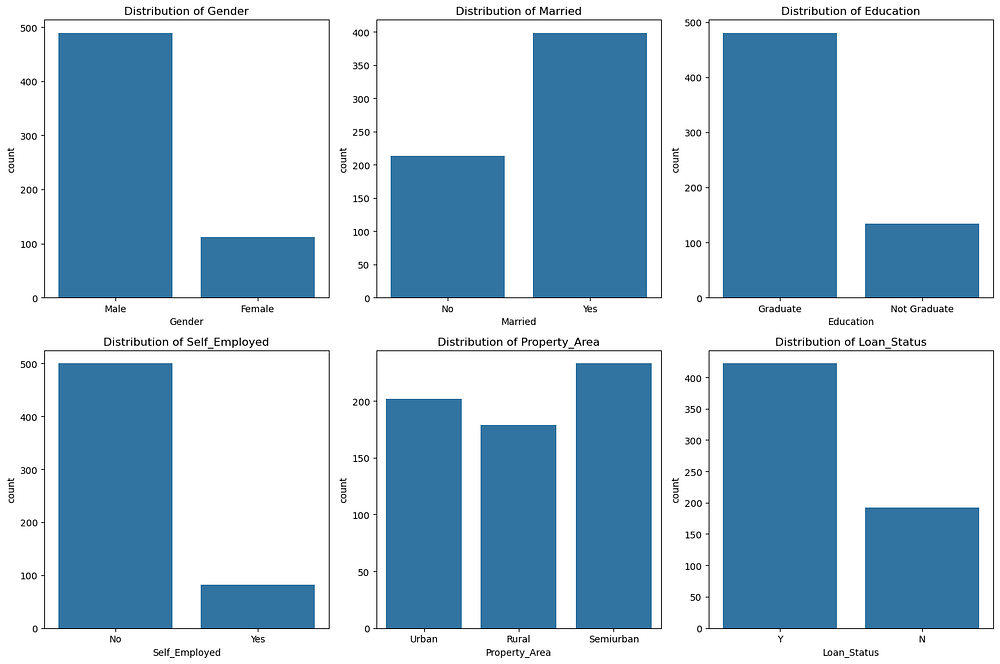
Gender: Most applicants are male, indicating a gender imbalance in the dataset.
Married: A higher proportion of applicants are married, which could influence loan approval.
Education: Graduates significantly outnumber non-graduates, suggesting education level may be an important feature.
Self-Employed: The majority of applicants are not self-employed, indicating a smaller representation of self-employed individuals.
Property_Area: Semiurban areas have the highest representation, followed by urban and rural areas.
Loan_Status: A larger proportion of loans are approved (
Y), indicating an imbalanced target variable.
These distributions suggest potential feature importance for predicting Loan_Status and highlight the need for strategies to address the imbalance in the target variable.
Distribution of Numerical Features
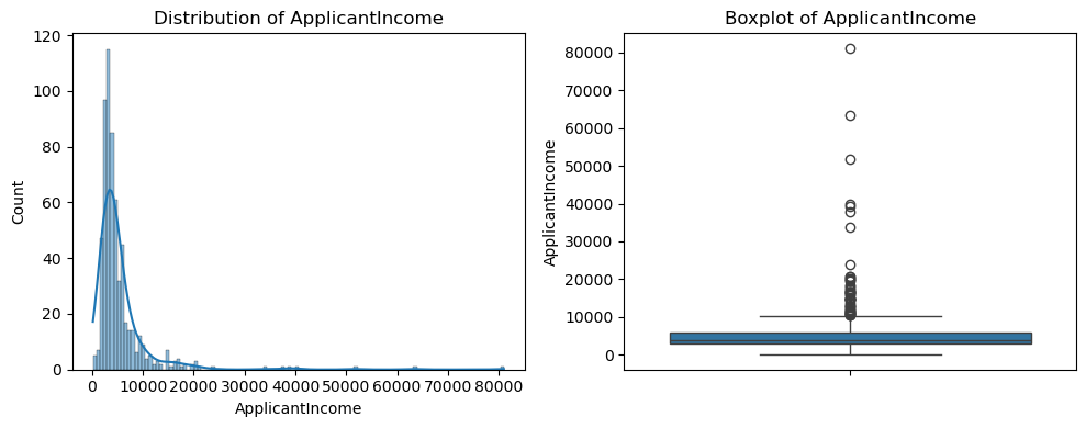
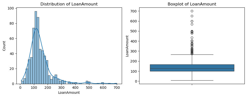
For numerical features like ApplicantIncome and LoanAmount, histograms and boxplots are used to examine their distribution and identify potential outliers:
# Plot numerical features
numerical_features = ['ApplicantIncome', 'CoapplicantIncome', 'LoanAmount']
for feature in numerical_features:
    plt.figure(figsize=(10, 4))

    # Histogram
    plt.subplot(1, 2, 1)
    sns.histplot(loan_data[feature], kde=True)
    plt.title(f'Distribution of {feature}')

    # Boxplot
    plt.subplot(1, 2, 2)
    sns.boxplot(loan_data[feature])
    plt.title(f'Boxplot of {feature}')

    plt.tight_layout()
    plt.show()
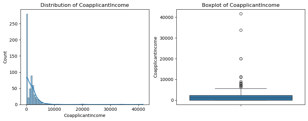
- CoapplicantIncome:
Distribution: Skewed towards 0, indicating many applicants have no co-applicant income.
Boxplot: Presence of extreme outliers beyond 10,000, which might affect model performance.
2. ApplicantIncome:
Distribution: Highly skewed to the right, with most values concentrated below 10,000.
Boxplot: Significant outliers above 20,000, suggesting a need for normalization or outlier handling.
3. LoanAmount:
Distribution: Right-skewed with most values between 100 and 200.
Boxplot: Outliers above 300, indicating variability in loan amounts applied for.
Overall, all three numerical features exhibit right-skewness and outliers. Moreover, feature scaling (e.g., standardization) and outlier handling may be necessary to improve model performance.
Correlation Analysis
Before analyzing correlations, we first check the unique values in the Dependents column and convert it to numerical format, as it contains ordinal data that is currently stored as an object. This ensures it can be included in the correlation matrix:
# Check unique values in the 'Dependents' column
print(loan_data['Dependents'].unique())
['0' '1' '2' '3+' nan]
# Convert 'Dependents' to numerical format
loan_data['Dependents'] = loan_data['Dependents'].replace({'3+': 3})
loan_data['Dependents'] = pd.to_numeric(loan_data['Dependents'], errors='coerce')
After converting and cleaning the Dependents column, we create a heatmap to analyze correlations between numerical features. This helps understand relationships within the data:
# Drop non-numerical or irrelevant columns
numerical_data = loan_data.select_dtypes(include=[np.number])

# Plot correlation heatmap
plt.figure(figsize=(10, 6))
sns.heatmap(numerical_data.corr(), annot=True, cmap='coolwarm')
plt.title('Correlation Matrix')
plt.show()
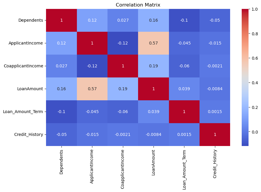
- Key Correlations:
ApplicantIncomeandLoanAmounthave a moderate positive correlation (0.57), indicating higher income applicants tend to apply for larger loans.Other correlations between features are generally weak or negligible.
Independence of Features: Most features, such as
Dependents,CoapplicantIncome, andCredit_History, show minimal correlation with each other, reducing concerns about multicollinearity.Target Variable (Loan_Status): Although not included in this heatmap, correlations with
Credit_History(a critical feature in loan approval) should be examined in further analysis.
Overall, ApplicantIncome and LoanAmount stand out with a moderate correlation, suggesting their importance in the dataset. However, weak correlations among other features indicate potential non-linear relationships worth exploring during model training.
4. Data Preprocessing
Effective preprocessing ensures the dataset is ready for model training. The following steps are performed:
Handling Missing Values
Missing values in features such as Gender, Married, Self_Employed, and LoanAmount are imputed:
# Fill missing categorical values with mode
for column in ['Gender', 'Married', 'Self_Employed']:
    loan_data[column].fillna(loan_data[column].mode()[0], inplace=True)

# Fill missing numerical values with median
loan_data['LoanAmount'].fillna(loan_data['LoanAmount'].median(), inplace=True)
loan_data['Loan_Amount_Term'].fillna(loan_data['Loan_Amount_Term'].median(), inplace=True)
loan_data['Credit_History'].fillna(loan_data['Credit_History'].mode()[0], inplace=True)
Encoding Categorical Features
One-hot encoding is used for categorical columns to avoid implying any order:
loan_data = pd.get_dummies(loan_data, columns=['Gender', 'Married', 'Education', 'Self_Employed', 'Property_Area'], drop_first=True)
Feature Scaling
Numerical features are scaled using StandardScaler for consistent range:
from sklearn.preprocessing import StandardScaler

scaler = StandardScaler()
scaled_features = scaler.fit_transform(loan_data[['ApplicantIncome', 'CoapplicantIncome', 'LoanAmount', 'Loan_Amount_Term']])
scaled_df = pd.DataFrame(scaled_features, columns=['ApplicantIncome', 'CoapplicantIncome', 'LoanAmount', 'Loan_Amount_Term'])
loan_data.update(scaled_df)
Splitting the Dataset
The data is split into training and testing sets, with the Loan_Status column as the target variable:
from sklearn.model_selection import train_test_split

X = loan_data.drop(columns=['Loan_ID', 'Loan_Status'])
y = loan_data['Loan_Status'].map({'Y': 1, 'N': 0})  # Convert target to binary
X_train, X_test, y_train, y_test = train_test_split(X, y, test_size=0.2, random_state=42)
5. Model Training
We train two models: Logistic Regression and Support Vector Machine (SVM), and compare their performance.
Logistic Regression
Logistic Regression is trained on the preprocessed data:
from sklearn.linear_model import LogisticRegression

log_reg = LogisticRegression()
log_reg.fit(X_train, y_train)
Support Vector Machine (SVM)
from sklearn.svm import SVC

svm_model = SVC(probability=True)  # Enable probability estimates for ROC curve
svm_model.fit(X_train, y_train)
Evaluating the Models
Both models are evaluated using accuracy, precision, recall, and F1-score:
from sklearn.metrics import classification_report

# Logistic Regression Performance
print("Logistic Regression Performance:")
print(classification_report(y_test, log_reg.predict(X_test)))

# SVM Performance
print("SVM Performance:")
print(classification_report(y_test, svm_model.predict(X_test)))
Logistic Regression Performance:
              precision    recall  f1-score   support

           0       0.95      0.42      0.58        43
           1       0.76      0.99      0.86        80

    accuracy                           0.79       123
   macro avg       0.85      0.70      0.72       123
weighted avg       0.83      0.79      0.76       123

SVM Performance:
              precision    recall  f1-score   support

           0       0.90      0.42      0.57        43
           1       0.76      0.97      0.85        80

    accuracy                           0.78       123
   macro avg       0.83      0.70      0.71       123
weighted avg       0.81      0.78      0.75       123
- Logistic Regression:
Class 1 (Loan Approved): High recall (0.99) indicates it correctly identifies most approved loans but at the cost of precision (0.76), meaning it misclassifies some rejected loans as approved.
Class 0 (Loan Rejected): Low recall (0.42) indicates it struggles to identify rejected loans, resulting in lower performance for this class.
Overall Accuracy: 79%, with a weighted F1-score of 0.76.
2. SVM:
Class 1 (Loan Approved): Similar to Logistic Regression, it achieves high recall (0.97) and a decent precision (0.76).
Class 0 (Loan Rejected): Slightly better precision (0.90) but equally low recall (0.42), indicating difficulty in handling this minority class.
Overall Accuracy: 78%, with a weighted F1-score of 0.75.
Overall:
Both models perform well in predicting approved loans (
Class 1) but struggle with rejected loans (Class 0) due to imbalanced data.Logistic Regression has slightly higher overall accuracy and weighted F1-score than SVM, but the difference is minimal.
Addressing the class imbalance (e.g., using SMOTE or class weighting) could improve performance, especially for rejected loans.
6. Model Fine-Tuning
To improve the model’s performance, especially in handling the imbalance between approved (Class 1) and rejected (Class 0) loans, we apply techniques like SMOTE (Synthetic Minority Oversampling Technique) and class weighting on the Logistics model since it has slightly better performance than the SVM model.
Using SMOTE
SMOTE generates synthetic samples for the minority class to balance the dataset:
from imblearn.over_sampling import SMOTE

# Apply SMOTE to the training set
smote = SMOTE(random_state=42)
X_train_smote, y_train_smote = smote.fit_resample(X_train, y_train)

# Train Logistic Regression on SMOTE data
log_reg_smote = LogisticRegression()
log_reg_smote.fit(X_train_smote, y_train_smote)

# Evaluate the model
print("Logistic Regression with SMOTE Performance:")
print(classification_report(y_test, log_reg_smote.predict(X_test)))
Logistic Regression with SMOTE Performance:
              precision    recall  f1-score   support

           0       0.81      0.49      0.61        43
           1       0.77      0.94      0.85        80

    accuracy                           0.78       123
   macro avg       0.79      0.71      0.73       123
weighted avg       0.79      0.78      0.76       123
Logistic Regression with SMOTE:
Class 0 (Rejected Loans): Precision (0.81) is good, but recall is low (0.49), meaning many rejected loans are still misclassified.
Class 1 (Approved Loans): High recall (0.94) and decent precision (0.77) indicate most approved loans are correctly identified.
Overall: Accuracy (0.78) is comparable to the baseline model, but recall for Class 0 remains a challenge.
Using Class Weighting
Class weighting adjusts the importance of each class during training to penalize misclassification of the minority class:
# Train Logistic Regression with class weighting
log_reg_weighted = LogisticRegression(class_weight='balanced')
log_reg_weighted.fit(X_train, y_train)

# Evaluate the model
print("Logistic Regression with Class Weighting Performance:")
print(classification_report(y_test, log_reg_weighted.predict(X_test)))
Logistic Regression with Class Weighting Performance:
              precision    recall  f1-score   support

           0       0.76      0.51      0.61        43
           1       0.78      0.91      0.84        80

    accuracy                           0.77       123
   macro avg       0.77      0.71      0.73       123
weighted avg       0.77      0.77      0.76       123
Logistic Regression with Class Weighting:
Class 0 (Rejected Loans): Lower precision (0.76) and recall (0.51) compared to SMOTE.
Class 1 (Approved Loans): Slightly lower recall (0.91) than SMOTE, but similar precision (0.78).
Overall: Accuracy (0.77) is slightly lower than SMOTE, with balanced performance across classes.
Overall:
SMOTE achieves better precision for Class 0, making it more suitable when minimizing false positives for rejected loans.
Class Weighting balances performance across both classes but with slightly lower precision for Class 0.
Both techniques improve overall model robustness but still face challenges in Class 0 recall due to inherent data imbalance.
7. Conclusion
In this project, we explored loan status prediction using machine learning with Logistic Regression and Support Vector Machines (SVM). Through detailed data preprocessing, including scaling and one-hot encoding, we prepared the dataset for effective modelling. Despite the class imbalance, the baseline models achieved good accuracy but struggled with rejected loan predictions (Class 0).
To address this, we applied fine-tuning techniques such as SMOTE and class weighting. These methods improved the model’s ability to handle the minority class, though challenges with Class 0 recall remained. Logistic Regression with SMOTE offered the best balance between precision and recall, making it the preferred model for this dataset.
This project highlights the importance of handling class imbalances and choosing the right techniques for specific business goals. Future work could explore advanced methods, such as ensemble learning or hyperparameter optimization, to further enhance model performance.
Appendices
Data source: https://www.kaggle.com/datasets/ninzaami/loan-predication
