1. Introduction to Fintech Case Study

In today’s fast-paced digital landscape, financial technology (FinTech) companies are leveraging data-driven insights to drive customer engagement and boost subscription conversions. With the rise of mobile applications, companies across various industries are increasingly focused on analyzing user behavior to create effective, targeted marketing campaigns. This case study explores a typical scenario where a FinTech company aims to identify free app users who are less likely to subscribe to their paid services, thus allowing the company to focus marketing resources more strategically.

This project uses a simulated dataset reflecting real-world trends in user behavior, with patterns designed to resemble interactions often observed in the industry. While the data is artificially generated due to the proprietary nature of actual FinTech data, it follows realistic distributions and correlations to represent common user actions in mobile apps.

Through this case study, we’ll explore the entire process of preparing, analyzing, and modeling data to identify users at high risk of not subscribing. We’ll dive into essential stages of exploratory data analysis, feature engineering, model building, and validation using various machine learning and data processing techniques. By the end of this study, we aim to develop a predictive model that will empower FinTech companies to target specific segments of users with tailored offers, increasing conversion rates while minimizing unnecessary marketing expenses.

This analysis is valuable not only for FinTech companies but also for any subscription-based business with a mobile presence. Understanding how users interact with the app and predicting subscription likelihood can help optimize marketing efforts, maximize return on investment, and ultimately drive long-term customer engagement and growth.

2. Objective and Business Challenge

The primary objective of this case study is to build a predictive model that identifies which free app users are less likely to convert to paid subscribers. In the competitive landscape of FinTech, many companies provide free versions of their services to attract users, eventually converting them into paying customers through a subscription model. However, targeting all users indiscriminately with subscription offers can be costly and inefficient.

This is where app behavior analysis comes in. By analyzing users’ interactions within the first 24 hours of app use, we can gain insights into the actions that distinguish likely subscribers from those who may need additional marketing to convert. This focused approach allows the company to allocate marketing resources more effectively, concentrating efforts on users who are less inclined to subscribe without further incentive.

In this case study, the app belongs to a FinTech company that provides financial tracking tools. The app offers both a free version and a paid version with premium features. The goal is to target users of the free version with personalized marketing shortly after their free trial period ends. Using a predictive model based on the first 24 hours of app interaction, we can help the company identify high-risk users who are unlikely to subscribe, enabling them to deliver targeted offers, such as free trial extensions or limited-time discounts.

This targeted approach not only improves conversion rates but also reduces marketing costs by focusing efforts on users most likely to respond. The insights from this analysis have far-reaching implications, offering a framework that can be adapted across other subscription-based industries to refine customer segmentation and optimize marketing strategies.

3. Loading and Understanding the Datasets

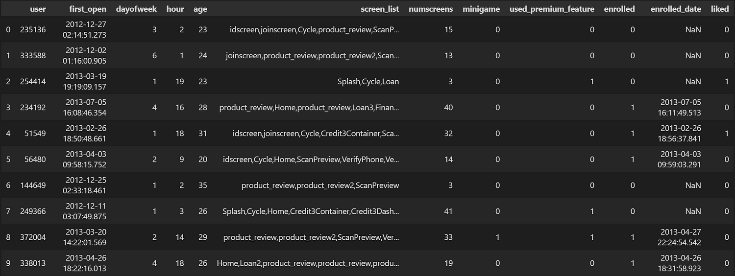
To effectively predict which users are likely to subscribe, it’s crucial to understand the data at hand. This dataset captures user behavior within the first 24 hours after they start using the app. The company focuses on this timeframe because the free trial period ends after 24 hours, making it essential to gather insights promptly to inform targeted marketing efforts. This early behavioral data helps build a model that can accurately identify potential subscribers and support proactive marketing strategies.

Key features in the dataset include:

User ID: A unique identifier for each user. While helpful for tracking individual users, this feature will be excluded from the model, as it holds no predictive value.
First Open: A timestamp recording the exact date and time each user initially opened the app. This allows us to analyze user activity relative to their initial app usage.
Day of the Week and Hour: These fields capture the specific day and hour when users first engaged with the app, offering insights into user behaviour patterns based on the time of access.
Age: The age of each user, which can reveal trends in subscription likelihood across different age demographics.
Screen List: This feature logs the specific screens each user visited within the app during the first 24 hours. The screen names are recorded as a comma-separated string, making this one of the most critical fields for analyzing engagement and interaction patterns.
Number of Screens Viewed: A count of the screens accessed by each user in the 24-hour period, giving a quick snapshot of each user’s engagement level.
Mini-Game Participation: Indicates whether a user engaged with an optional mini-game within the app. This is captured as a binary variable, with 1 meaning the user played the game and 0 meaning they did not.
Likes and used_premium_feature: These binary features show whether a user likes any content or access premium features during the free trial, providing additional context for user engagement levels.
Enrollment: The target variable for this analysis, where 1 indicates that a user converted to a paid subscriber and 0 means they did not. This label will be crucial for training the model to predict subscription likelihood.
Enroll Date: This timestamp records the date of enrollment, allowing us to calculate the time between the first app open and the subscription date, an important measure for understanding user decision timelines.

Each of these features contributes unique information to the dataset, offering insights into user engagement, behavioral patterns, and demographic differences. Together, they provide a solid foundation for developing a predictive model. The data’s focus on the first 24 hours is especially critical, as it aligns with the company’s marketing strategy of targeting users immediately after their free trial ends.

This is an overview of the dataset’s head:

import pandas as pd
from dateutil import parser
import matplotlib.pyplot as plt
import numpy as np
import seaborn as sn

dataset = pd.read_csv('appdata10.csv')
dataset.head(10) # Viewing the Data

Here is the dataset’s information:

# Features' information
dataset.info()

<class 'pandas.core.frame.DataFrame'>
RangeIndex: 50000 entries, 0 to 49999
Data columns (total 12 columns):
 #   Column                Non-Null Count  Dtype 
---  ------                --------------  ----- 
 0   user                  50000 non-null  int64 
 1   first_open            50000 non-null  object
 2   dayofweek             50000 non-null  int64 
 3   hour                  50000 non-null  int32 
 4   age                   50000 non-null  int64 
 5   screen_list           50000 non-null  object
 6   numscreens            50000 non-null  int64 
 7   minigame              50000 non-null  int64 
 8   used_premium_feature  50000 non-null  int64 
 9   enrolled              50000 non-null  int64 
 10  enrolled_date         31074 non-null  object
 11  liked                 50000 non-null  int64 
dtypes: int32(1), int64(8), object(3)
memory usage: 4.4+ MB

The dataset has some features categorized as ‘object’ datatype, we will convert these later in the feature engineering part.

Through initial data exploration and feature engineering, we’ll transform this data into actionable insights, refining the dataset to capture patterns that distinguish potential subscribers from non-subscribers. These insights will be essential as we progress toward building an effective predictive model.

4. Exploratory Data Analysis (EDA)

Before diving into model building, it’s essential to understand the data through exploratory data analysis (EDA). In this stage, we’ll examine the structure of the dataset, visualize key features, and analyze correlations that may impact subscription likelihood. By exploring patterns in user behaviour, we can identify the variables that provide the most predictive power for our model.

Visualizing Feature Distributions

We begin by plotting histograms for the primary numerical features in our dataset. These visualizations help us understand the data distribution and identify any skewness that could affect our model.

import matplotlib.pyplot as plt
import numpy as np

# Drop unnecessary columns for plotting
dataset2 = dataset.copy().drop(columns=['user', 'screen_list', 'enrolled_date', 'first_open', 'enrolled'])

# Plot histograms for numerical features
plt.suptitle('Histograms of Numerical Columns', fontsize=20)
for i in range(1, dataset2.shape[1] + 1):
    plt.subplot(3, 3, i)
    plt.hist(dataset2.iloc[:, i - 1], bins=np.size(dataset2.iloc[:, i - 1].unique()), color='#3F5D7D')
    plt.title(dataset2.columns.values[i - 1])
plt.tight_layout(rect=[0, 0.03, 1, 0.95])
plt.show()

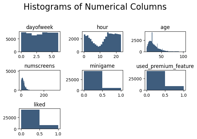
In the histograms:

Day of the Week and Hour: We see an even distribution across days, while the hour of initial app use shows a dip during early morning hours, indicating lower engagement late at night.
Age: Age is relatively evenly distributed, with slight peaks around ages 29 and 41, which could indicate higher engagement from these demographics.
Number of Screens Viewed: The average user views around 15–25 screens, with a few outliers showing unusually high or low engagement.

These histograms provide an initial look at user behavior, showing patterns that may impact subscription likelihood.

Correlation Analysis with Response Variable

Next, we analyze the correlation between each feature and the target variable, Enrollment. This helps us identify which features might have the strongest influence on a user’s decision to subscribe.

# Plot correlation with the response variable
dataset2.corrwith(dataset['enrolled']).plot.bar(
    figsize=(20, 10), title='Correlation with Response Variable', fontsize=15, rot=45, grid=True)
plt.show()

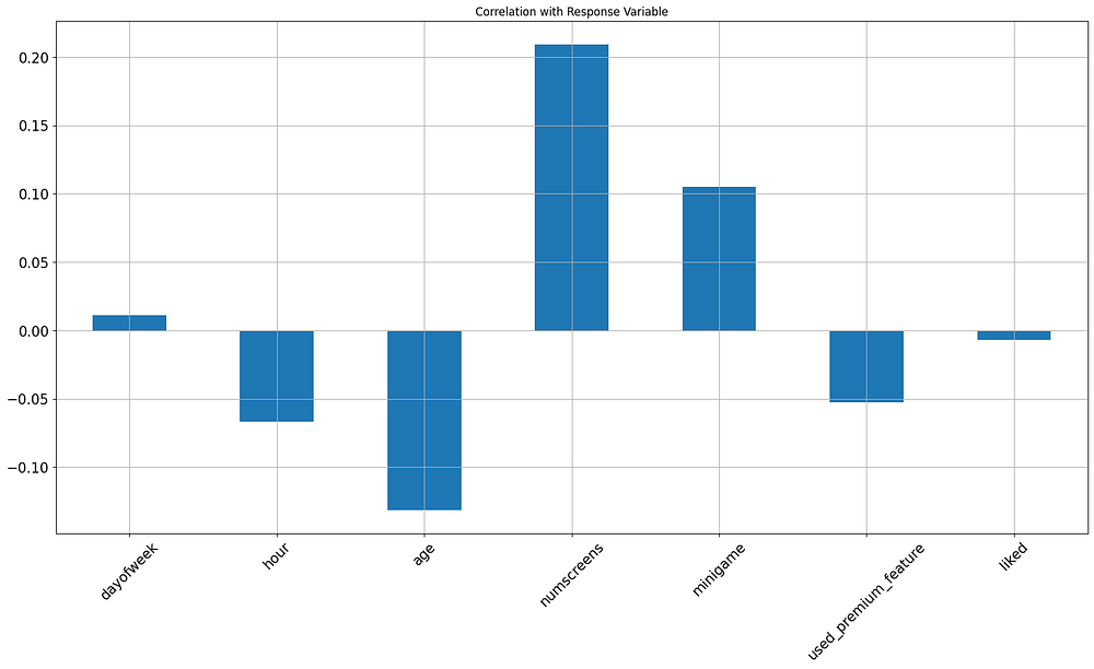
In this bar plot:

Positive Correlations: Higher num_screens viewed and mini_game engagement correlate with a greater likelihood of subscription, suggesting that more engaged users are more likely to convert.
Negative Correlations: A slight negative correlation with hour and age suggests that younger users and those engaging at certain times may be more inclined to subscribe.

These correlations provide useful insights into which features may be more predictive of user subscription behavior.

Correlation Matrix

To ensure our features are relatively independent, we generate a correlation matrix, which shows relationships between all numerical features. High correlations between independent variables could introduce multicollinearity, potentially affecting model performance.

# Compute the correlation matrix
corr = dataset2.corr()

# Generate a mask for the upper triangle
mask = np.triu(np.ones_like(corr, dtype=bool))

### Plot the heatmap
plt.figure(figsize=(18, 15))
sns.heatmap(corr, mask=mask, cmap=sns.diverging_palette(220, 10, as_cmap=True), center=0,
            square=True, linewidths=0.5, cbar_kws={"shrink": 0.5}, annot=True, fmt=".2f",
            annot_kws={'fontsize': 16})
plt.title("Correlation Matrix", fontsize=20)
plt.show()

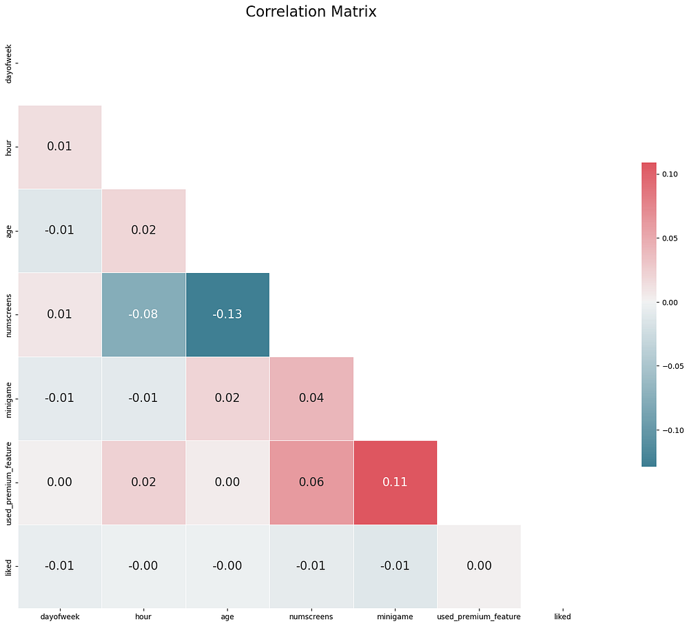
The heatmap shows low multicollinearity among most features, validating their independence. However, we do observe:

Screens Viewed and Premium Feature Usage: A moderate correlation, indicating that users who view more screens are also likely to engage with premium features.
Mini-Game and Premium Feature Usage: These features also show some correlation, suggesting that users who play the mini-game are more engaged with premium content.

These insights confirm the suitability of our features for modeling, as they exhibit only minimal dependencies on each other.

5. Feature Engineering

Feature engineering is a crucial step in preparing data for modeling. In this project, we refine several features to capture user behavior patterns that are likely to predict subscription likelihood. This involves transforming time-based features, encoding user interactions, and creating aggregated metrics based on app screen usage.

Engineering the Response Variable

The primary objective of this analysis is to predict whether a user will subscribe within a specified time window. Firstly, let’s plot the distribution of time since the enrollment of users:

# Plotting the distribution to confirm cutoff
plt.hist(dataset["difference"].dropna(), color='#3F5D7D')
plt.title('Distribution of Time-Since-Enrollment')
plt.xlabel('Time Since First Open (hours)')
plt.ylabel('Number of Users')
plt.show()

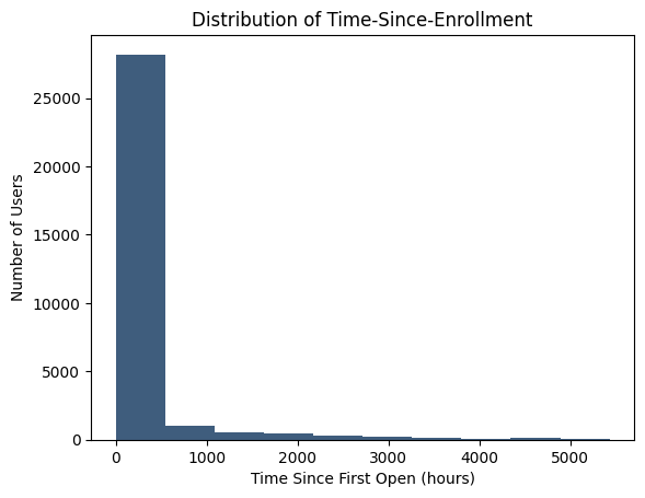
We can see that most users enrolled within the first 500 hours, we will dive deeper into the first 500 hours to get more insight:

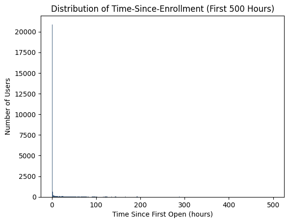
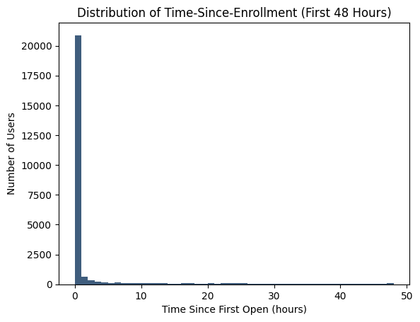
It seems like the user's enrollment again focuses mostly on the first few days. Based on this insight, we set a 48-hour threshold (2 days) for enrollment:

# Plotting the distribution within the first 48 hours
plt.hist(dataset["difference"].dropna(), bins=48, range=(0, 48), color='#3F5D7D')
plt.title('Distribution of Time-Since-Enrollment (First 48 Hours)')
plt.xlabel('Time Since First Open (hours)')
plt.ylabel('Number of Users')
plt.show()

# Setting cutoff for enrollment at 48 hours
dataset.loc[dataset.difference > 48, 'enrolled'] = 0
dataset = dataset.drop(columns=['enrolled_date', 'difference', 'first_open'])

This transformation converts users who enrolled after 48 hours to a non-enrollment status (0), simplifying our prediction goal to whether users convert within this timeframe.

Processing Screen List Data

The screen_list column in appdata10.csv contains a comma-separated list of screens that each user visited within the first 24 hours of using the app. This feature is critical for understanding user engagement with different parts of the app, as it allows us to track which specific screens were accessed. These are the unique values of the screen_list column:

# Display all unique values in the 'screen_list' column
unique_screens = dataset["screen_list"].str.split(',', expand=True).stack().unique()
unique_screens

['idscreen' 'joinscreen' 'Cycle' 'product_review' 'ScanPreview'
 'VerifyDateOfBirth' 'VerifyPhone' 'VerifyToken' 'ProfileVerifySSN'
 'Loan2' 'Settings' 'ForgotPassword' 'Login' 'product_review2' 'location'
 'VerifyCountry' 'Institutions' 'Splash' 'Loan' 'Home' 'Loan3' 'Finances'
 'Credit3' 'ReferralContainer' 'Leaderboard' 'Rewards' 'RewardDetail'
 'VerifySSN' 'Credit1' 'Credit2' 'Credit3Container' 'SelectInstitution'
 'BankVerification' 'Credit3Dashboard' 'product_review3' 'TransactionList'
 'RewardsContainer' 'Loan4' 'CC1' 'CC1Category' 'Alerts' 'ProfilePage'
 'CC3' 'MLWebView' 'GroupedInstitutions' 'ReferralScreen' 'ResendToken'
 'WebView' 'ProfileChildren' 'ProfileEducation' 'ProfileEducationMajor'
 'Saving9' 'Saving1' 'VerifyMobile' 'LoginForm' 'BVPlaidLinkContainer'
 'Saving10' 'Saving4' 'Saving7' 'Saving6' 'Saving5' 'VerifyHousing'
 'VerifyHousingAmount' 'Saving8' 'CommunityAndInvites' 'SavingGoalPreview'
 'SavingGoalEdit' 'EditProfile' 'ProfileMaritalStatus' 'VerifyBankInfo'
 'VerifyIncomeType' 'ProfileJobTitle' 'ProfileCompanyName'
 'ProfileEmploymentLength' 'Rewardjoinscreen' 'Loan1' 'Credit3Alerts'
 'VerifyAnnualIncome' 'LandingScreen' 'Saving2' 'ListPicker' 'About'
 'FindFriendsCycle' 'WelcomeBankVerification' 'ManageFinances'
 'AccountView' 'History' 'SecurityModal' 'Saving2Amount'
 'Profileproduct_review' 'SavingGoalIncomeSalary'
 'ProfileVerifyIncomeType' 'ProfileAnnualIncome' 'SignupName' 'Signup'
 'NetworkFailure' 'LoanAppScheduleCall' 'product_review5'
 'product_review4' 'LoanAppRequestAmount' 'LoanAppReasons'
 'ContactInfoConfirm' 'LoanAppPromoCode' 'LoanAppAgreement'
 'LoanAppDenied' 'LLLoanAmount' 'LoanAppESign' 'LoanAppPaymentSchedule'
 'LoanAppSuccess' 'SavingGoalOther' 'NewContactListInvite' 'Payoff'
 'CameraScreen' 'EmploymentSummary' 'Referrals' 'YourNetwork'
 'LoanAppBankInfo' 'SignupEmail' 'AddVehicle' 'ReviewCreditCard'
 'AddProperty' 'InstantOfferCreateAccount' 'Credits' 'EmploymentInfo'
 'BVStats' 'BoostFriendsList' 'LoanAppConfirmWithdrawal' 'AdverseActions'
 'LoanAppWithdrawn' 'ProviderList' 'IdentityVerification'
 'LoanAppVerifyBankInfo' 'LoanAppLoan4' 'NetworkUser' 'Credit3CTA'
 'InstantLoanSSN' 'IdAndSelfieCameraScreen']

Instead of treating screen_list as a single column, we extract specific screens into high-level "funnels" to capture broader engagement patterns. These funnels focus on important app functionalities, like savings, credit, and loans, which are most relevant to predicting subscription likelihood.

Why Only Select Screens Were Grouped?

Not all screens in screen_list were included in the funnel creation process. Here’s why:

Relevance to Subscription Prediction: Screens related to financial actions, such as loans, credit, and savings, are likely more predictive of subscription likelihood than screens unrelated to monetization, like profile settings or community engagement. By focusing on these relevant screens, we increase the effectiveness of our model.
Reducing Complexity: Including every screen as a separate feature or attempting to create funnels for all of them would add unnecessary complexity, increasing the risk of overfitting and potentially diluting the predictive power of key features. By selecting only a subset of screens, we keep the dataset manageable and focused.
Alignment with Business Objectives: The selected funnels (e.g., savings, credit, and loans) reflect key functionalities that align with the app’s business objectives and revenue-driving actions. These categories help capture user interactions that are meaningful from a business perspective, potentially correlating with users who are more likely to convert to paid subscribers.

Aggregating Screens into Funnels

Based on this selection process, we created funnel features by aggregating screens that fall within each category. For example, screens related to the savings feature (such as Saving1, Saving2, etc.) are aggregated into a SavingCount feature, which counts how many times a user interacted with savings-related screens.

These funnel features (e.g., SavingCount, CMCount, CCCount, and LoansCount) capture engagement with major app sections. Aggregating in this way reduces complexity, allowing the model to generalize more effectively across similar user actions.

# Aggregating screens into funnels
appdata10["SavingCount"] = appdata10["screen_list"].apply(lambda x: sum(screen in x for screen in savings_screens))
appdata10["CMCount"] = appdata10["screen_list"].apply(lambda x: sum(screen in x for screen in credit_screens))
appdata10["CCCount"] = appdata10["screen_list"].apply(lambda x: sum(screen in x for screen in cc_screens))
appdata10["LoansCount"] = appdata10["screen_list"].apply(lambda x: sum(screen in x for screen in loan_screens))
appdata10.info()

<class 'pandas.core.frame.DataFrame'>
RangeIndex: 50000 entries, 0 to 49999
Data columns (total 72 columns):
 #   Column                   Non-Null Count  Dtype
---  ------                   --------------  -----
 0   user                     50000 non-null  int64
 1   dayofweek                50000 non-null  int64
 2   hour                     50000 non-null  int32
 3   age                      50000 non-null  int64
 4   numscreens               50000 non-null  int64
 5   minigame                 50000 non-null  int64
 6   used_premium_feature     50000 non-null  int64
 7   enrolled                 50000 non-null  int64
 8   liked                    50000 non-null  int64
 9   SavingCount              50000 non-null  int64
 10  CMCount                  50000 non-null  int64
 11  CCCount                  50000 non-null  int64
 12  LoansCount               50000 non-null  int64
 13  Loan2                    50000 non-null  int32
 14  location                 50000 non-null  int32
 15  Institutions             50000 non-null  int32
 16  Credit3Container         50000 non-null  int32
 17  VerifyPhone              50000 non-null  int32
 18  BankVerification         50000 non-null  int32
 19  VerifyDateOfBirth        50000 non-null  int32
 20  ProfilePage              50000 non-null  int32
 21  VerifyCountry            50000 non-null  int32
 22  Cycle                    50000 non-null  int32
 23  idscreen                 50000 non-null  int32
 24  Credit3Dashboard         50000 non-null  int32
 25  Loan3                    50000 non-null  int32
 26  CC1Category              50000 non-null  int32
 27  Splash                   50000 non-null  int32
 28  Loan                     50000 non-null  int32
 29  CC1                      50000 non-null  int32
 30  RewardsContainer         50000 non-null  int32
 31  Credit3                  50000 non-null  int32
 32  Credit1                  50000 non-null  int32
 33  EditProfile              50000 non-null  int32
 34  Credit2                  50000 non-null  int32
 35  Finances                 50000 non-null  int32
 36  CC3                      50000 non-null  int32
 37  Saving9                  50000 non-null  int32
 38  Saving1                  50000 non-null  int32
 39  Alerts                   50000 non-null  int32
 40  Saving8                  50000 non-null  int32
 41  Saving10                 50000 non-null  int32
 42  Leaderboard              50000 non-null  int32
 43  Saving4                  50000 non-null  int32
 44  VerifyMobile             50000 non-null  int32
 45  VerifyHousing            50000 non-null  int32
 46  RewardDetail             50000 non-null  int32
 47  VerifyHousingAmount      50000 non-null  int32
 48  ProfileMaritalStatus     50000 non-null  int32
 49  ProfileChildren          50000 non-null  int32
 50  ProfileEducation         50000 non-null  int32
 51  Saving7                  50000 non-null  int32
 52  ProfileEducationMajor    50000 non-null  int32
 53  Rewards                  50000 non-null  int32
 54  AccountView              50000 non-null  int32
 55  VerifyAnnualIncome       50000 non-null  int32
 56  VerifyIncomeType         50000 non-null  int32
 57  Saving2                  50000 non-null  int32
 58  Saving6                  50000 non-null  int32
 59  Saving2Amount            50000 non-null  int32
 60  Saving5                  50000 non-null  int32
 61  ProfileJobTitle          50000 non-null  int32
 62  Login                    50000 non-null  int32
 63  ProfileEmploymentLength  50000 non-null  int32
 64  WebView                  50000 non-null  int32
 65  SecurityModal            50000 non-null  int32
 66  Loan4                    50000 non-null  int32
 67  ResendToken              50000 non-null  int32
 68  TransactionList          50000 non-null  int32
 69  NetworkFailure           50000 non-null  int32
 70  ListPicker               50000 non-null  int32
 71  Other                    50000 non-null  int64
dtypes: int32(59), int64(13)
memory usage: 16.2 MB

Creating the ‘Other’ Feature

To capture user engagement with app screens outside our primary categories (savings, credit, credit card, and loan screens), we created a feature called Other. This feature represents the number of screens a user interacts with that does not fall into one of the four main screen categories.

First, we convert each entry in the screen_list column from a comma-separated string into a list of individual screens. This allows us to easily filter out screens that belong to our defined categories and count only the remaining screens in each list.

# Convert screen_list column to a list of screens for each entry
dataset["screen_list"] = dataset["screen_list"].apply(lambda x: x.split(','))

# Define screen categories
savings_screens = ["Saving1", "Saving2", "Saving2Amount", "Saving4", "Saving5", "Saving6", "Saving7", "Saving8", "Saving9", "Saving10"]
credit_screens = ["Credit1", "Credit2", "Credit3", "Credit3Container", "Credit3Dashboard"]
cc_screens = ["CC1", "CC1Category", "CC3"]
loan_screens = ["Loan", "Loan2", "Loan3", "Loan4"]

# Combine all category screens into one list for filtering
all_category_screens = savings_screens + credit_screens + cc_screens + loan_screens

# Filter out category screens and count remaining screens for the 'Other' feature
dataset["Other"] = dataset["screen_list"].apply(lambda screens: sum(screen not in all_category_screens for screen in screens))

# Drop the screen_list column as it’s no longer needed
dataset = dataset.drop(columns=["screen_list"])

In this code:

screen_list Conversion: The apply(lambda x: x.split(',')) line converts each screen_list entry into a list, where each screen name becomes a separate item in the list.
Category Screen Removal: We define the four screen categories (savings_screens, credit_screens, cc_screens, loan_screens) and combine them into a single list called all_category_screens.
Counting “Other” Screens: For each user’s screen_list, we count the screens that do not belong to any of the four categories, using a generator expression inside sum(). This count is stored in the Other column.
Dropping screen_list: Finally, we drop the screen_list column since it’s no longer needed after the creation of the Other feature.

The Other feature now represents the total number of screens a user visited outside the primary screen categories. This feature can provide insight into users’ general engagement with miscellaneous or less prominent screens, offering an additional metric that may help the model understand broader app usage patterns.

6. Data Preprocessing

With the exploratory data analysis (EDA) and feature engineering completed in EDA.py, we now have a clean, structured dataset saved as processed_appdata10.csv. This dataset includes essential transformations such as:

Conversion of timestamps into time-based features,
Creation of engagement funnels for major app features (e.g., Savings, Credit),
Calculation of relevant metrics like SavingCount, CMCount, CCCount, and LoansCount, and
Cleaning and extraction of high-level screen engagement metrics.

The next steps in our analysis take place in a new module, Model.py, which focuses solely on data preprocessing for modeling, train-test splitting, and building the machine learning model.

Loading the Processed Dataset

The final, preprocessed dataset is loaded directly in Model.py:

import pandas as pd

# Load the dataset processed in EDA.py
dataset = pd.read_csv("processed_appdata10.csv")

Splitting the Data for Training and Testing

To evaluate our model’s performance effectively, we split the dataset into training and testing sets. This helps in testing the model’s accuracy on unseen data after it has been trained.

from sklearn.model_selection import train_test_split

# Define the response variable and features
X = dataset.drop(columns=['enrolled'])  # Dropping the target variable from features
y = dataset['enrolled']  # Defining the target variable

# Perform the train-test split
X_train, X_test, y_train, y_test = train_test_split(X, y, test_size=0.2, random_state=0)

In this code:

X includes all features in the dataset except for enrolled, which is the target variable.
y contains only the target variable, enrolled, which indicates whether a user converted to a paid subscription.
We use an 80/20 split ratio to allocate 80% of the data for training and 20% for testing.

Removing Identifiers

To maintain data privacy and ensure model integrity, we remove the user identifier column from our training and testing data. Although the user ID uniquely identifies each user, it doesn’t provide any predictive information and could introduce noise into the model. We save the user identifiers separately to link predictions back to users after the model is built:

# Removing Identifiers
train_identity = X_train['user']
X_train = X_train.drop(columns=['user'])
test_identity = X_test['user']
X_test = X_test.drop(columns=['user'])

Scaling the Features

For effective model performance, especially with algorithms sensitive to feature scaling (such as logistic regression), we apply standard scaling to ensure all features have similar ranges.

from sklearn.preprocessing import StandardScaler

# Initialize the scaler
scaler = StandardScaler()

# Fit and transform the training features, then transform the testing features
X_train = scaler.fit_transform(X_train)
X_test = scaler.transform(X_test)

7. Model Building and Evaluation

With the data preprocessed and feature-engineered, we’re ready to build and evaluate our model. In this project, we use logistic regression as our classification model to predict the likelihood of users subscribing to the paid version of the app. Logistic regression is effective for binary classification tasks and provides interpretable results.

Step 1: Training the Model

We start by importing and initializing the logistic regression model from scikit-learn. By setting the penalty parameter to 'l1', we apply L1 regularization (also known as Lasso regularization), which helps to reduce the influence of less relevant features, improving model interpretability and potentially reducing overfitting.

from sklearn.linear_model import LogisticRegression

# Initialize logistic regression model with L1 regularization
model = LogisticRegression(penalty='l1', solver='saga', random_state=0)
model.fit(X_train, y_train)

Step 2: Making Predictions

After training the model on the training dataset, we make predictions on the test dataset to assess its performance on unseen data.

# Make predictions on the test set
y_pred = model.predict(X_test)

Step 3: Evaluating Model Performance

To measure the effectiveness of our model, we calculate several evaluation metrics:

from sklearn.metrics import accuracy_score, precision_score, recall_score, f1_score

# Calculate evaluation metrics
accuracy = accuracy_score(y_test, y_pred)
precision = precision_score(y_test, y_pred)
recall = recall_score(y_test, y_pred)
f1 = f1_score(y_test, y_pred)

# Print the results
print(f"Accuracy: {accuracy:.2f}")
print(f"Precision: {precision:.2f}")
print(f"Recall: {recall:.2f}")
print(f"F1 Score: {f1:.2f}")

Accuracy: 0.73
Precision: 0.73
Recall: 0.72
F1 Score: 0.72

The model performs reasonably well, with an Accuracy of 73%, indicating that it correctly predicts subscription status 73% of the time.

Precision (0.73): Of the users predicted to subscribe, 73% actually did, showing that the model is fairly precise in identifying likely subscribers.
Recall (0.72): The model correctly identifies 72% of actual subscribers, meaning it captures a good portion of true subscribers but misses some.
F1 Score (0.72): The F1 Score, a balance between precision and recall, is 0.72, suggesting that the model has a well-balanced ability to identify subscribers without too many false positives or negatives.

Overall, these metrics indicate a moderately effective model, suitable for guiding targeted marketing efforts but with room for improvement in capturing all true subscribers.

Step 4: Confusion Matrix

A confusion matrix offers a detailed view of the model’s performance by displaying the counts of true positive, true negative, false positive, and false negative predictions. This breakdown provides insight into specific types of errors, such as predicting a non-subscriber as a subscriber.

from sklearn.metrics import confusion_matrix
import seaborn as sns
import matplotlib.pyplot as plt

# Create and plot the confusion matrix
conf_matrix = confusion_matrix(y_test, y_pred)
sns.heatmap(conf_matrix, annot=True, fmt="d", cmap="Blues", xticklabels=["Non-Subscriber", "Subscriber"], yticklabels=["Non-Subscriber", "Subscriber"])
plt.xlabel("Predicted Label")
plt.ylabel("True Label")
plt.title("Confusion Matrix")
plt.show()

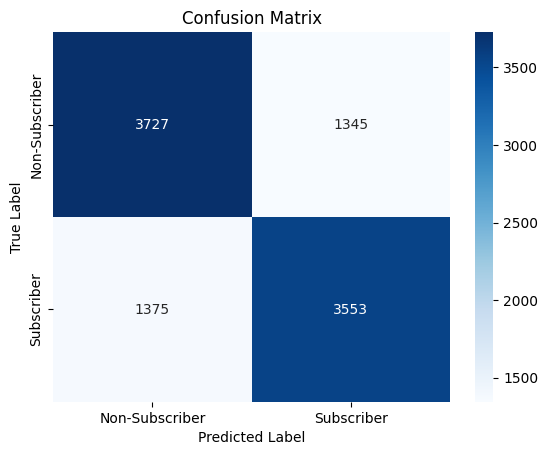
The confusion matrix indicates the following:

True Negatives (Non-Subscribers correctly predicted): 3,727
False Positives (Non-Subscribers incorrectly predicted as Subscribers): 1,345
False Negatives (Subscribers incorrectly predicted as Non-Subscribers): 1,375
True Positives (Subscribers correctly predicted): 3,553

This shows that the model performs relatively well, but there are some misclassifications, especially with false positives and false negatives, which slightly reduce the model’s precision and recall.

Step 5: Cross-Validation for Model Reliability

To ensure the robustness of our model, we use k-fold cross-validation with k=10, which splits the data into 10 subsets, trains the model on 9 subsets, and tests on the remaining subset. This process is repeated for all subsets, and the results are averaged to provide a reliable measure of the model’s performance.

# Applying k-Fold Cross Validation
from sklearn.model_selection import cross_val_score

# Perform 10-fold cross-validation
cv_scores = cross_val_score(model, X_train, y_train, cv=10, scoring='accuracy')
print(f"Cross-Validation Accuracy: {cv_scores.mean():.2f} ± {cv_scores.std() * 2:.2f}")

Cross-Validation Accuracy: 0.72 ± 0.02

The cross-validation accuracy of 72% ± 2% indicates that the model consistently performs with around 72% accuracy across different data splits, with only a small variation (2%). This suggests the model is stable and generalizes well to new data.

Summary of Results

The model’s evaluation metrics demonstrate its effectiveness in predicting user subscriptions. With an accuracy of 73%, precision of 73%, recall of 72%, and F1 score of 0.72, the model shows a balanced ability to distinguish between subscribers and non-subscribers, though it does miss some true subscribers and occasionally misclassifies non-subscribers as subscribers.

The cross-validation accuracy of 72% ± 2% further confirms the model’s consistency and reliability across different data splits, indicating stable performance.

By leveraging logistic regression with L1 regularization and a thorough evaluation, we have built a model that can effectively identify potential subscribers, supporting more targeted marketing efforts and potentially increasing subscription rates for the business.

8. Hyperparameter Tuning

To further improve the performance of our logistic regression model, we perform hyperparameter tuning. This process involves optimizing key parameters to find the best configuration for the model, which can help enhance accuracy, precision, and other performance metrics.

For logistic regression, we tune parameters like:

Penalty (penalty): Regularization technique used to prevent overfitting. We typically choose between l1 (Lasso) and l2 (Ridge) regularization.
Regularization Strength (C): Controls the degree of regularization, where a lower C increases regularization strength.
Solver (solver): Algorithm used for optimization. Different solvers work better with different penalties and dataset sizes (e.g., liblinear, saga).

We use Grid Search Cross-Validation to systematically try different combinations of these hyperparameters and identify the best configuration.

Implementing Grid Search

To fine-tune our logistic regression model, we perform hyperparameter tuning with two rounds of Grid Search. This two-step approach allows us to first conduct a broad search over a wider range of values for the regularization strength parameter (C), then narrow down to a more specific range based on the initial results.

Round 1 focuses on a broader range to identify the general area where optimal values might lie, while Round 2 performs a finer search to precisely tune the model.

from sklearn.model_selection import GridSearchCV
from sklearn.linear_model import LogisticRegression
import time

# Initialize logistic regression model
classifier = LogisticRegression(random_state=0)

### Grid Search - Round 1 ###

# Define broad hyperparameter grid for Round 1
param_grid_round1 = {
    'penalty': ['l1', 'l2'],
    'C': [0.001, 0.01, 0.1, 1, 10, 100, 1000]
}

# Set up GridSearchCV
grid_search1 = GridSearchCV(estimator=classifier, param_grid=param_grid_round1, scoring='accuracy', cv=10, n_jobs=-1)

# Run Grid Search and time the process
t0 = time.time()
grid_search1.fit(X_train, y_train)
t1 = time.time()
print(f"Round 1 took {t1 - t0:.2f} seconds")

# Capture the best parameters from Round 1
best_params_round1 = grid_search1.best_params_
print(f"Best Parameters from Round 1: {best_params_round1}")

Round 1 took 0.94 seconds
Best Parameters from Round 1: {'C': 0.1, 'penalty': 'l2'}

### Grid Search - Round 2 ###

# Define focused hyperparameter grid based on Round 1 results
param_grid_round2 = {
    'penalty': ['l1', 'l2'],
    'C': [0.1, 0.5, 0.9, 1, 2, 5]  # Narrowed range around the best values from Round 1
}

# Set up GridSearchCV for Round 2
grid_search2 = GridSearchCV(estimator=classifier, param_grid=param_grid_round2, scoring='accuracy', cv=10, n_jobs=-1)

# Run Grid Search and time the process
t0 = time.time()
grid_search2.fit(X_train, y_train)
t1 = time.time()
print(f"Round 2 took {t1 - t0:.2f} seconds")

# Capture the best parameters and model from Round 2
best_params = grid_search2.best_params_
best_model = grid_search2.best_estimator_

print(f"Best Parameters from Round 2: {best_params}")

Round 2 took 0.86 seconds
Best Parameters from Round 2: {'C': 0.5, 'penalty': 'l2'}

The two-round Grid Search process was efficient, taking less than a second for each round. In Round 1, the best parameters were identified as C = 0.1 and penalty = 'l2', guiding a more focused search in Round 2. In Round 2, the optimal parameters were refined to C = 0.5 with penalty = 'l2', providing the final configuration for the model. This indicates that the model performs best with moderate regularization (C = 0.5) using L2 regularization.

9. Conclusion and Business Impact

In this project, we successfully built and optimized a logistic regression model to predict user subscriptions based on app behavior. Through thorough preprocessing, feature engineering, and hyperparameter tuning, the model achieved a balanced performance, with an accuracy of 73%, precision of 73%, and recall of 72%. These results indicate that the model effectively identifies users likely to subscribe while maintaining a good balance between precision and recall.

Business Impact

The model provides valuable insights for targeted marketing strategies:

Targeted Marketing: By focusing on users identified as likely to subscribe, marketing campaigns can be more precisely directed, potentially increasing subscription rates while reducing unnecessary outreach costs.
Resource Optimization: Marketing resources can be allocated more efficiently by minimizing efforts on users unlikely to convert, allowing the business to invest in high-value customers.
Strategic Offers: The model enables the business to identify segments that may benefit from special offers or retention strategies, enhancing the overall customer journey.

This predictive framework supports data-driven decision-making, helping the business maximize its subscription growth and optimize marketing ROI. With potential for further refinement, this model serves as a foundation for improving user engagement and enhancing profitability through effective user targeting.

Appendices

Code: https://github.com/Minhhoang2606/Machine-learning-practical/tree/main/3.%20Directing%20customers%20to%20subscription%20through%20app%20behavior%20analysis

Data source: https://www.kaggle.com/datasets/raghavraipuria/fintech-data

Directing Customers to Subscription Through App Behavior Analysis with Logistic Regression

Table of contents