1. Introduction

Predicting customer purchase behaviors is a crucial aspect of modern business intelligence. In this project, we aim to predict the car purchase amount of customers using a machine learning approach. By leveraging historical customer data, businesses like car dealerships can tailor their marketing strategies and better understand customer spending patterns.

The dataset used for this project includes detailed customer information such as age, income, credit card debt, and other financial metrics. Through this analysis, we not only aim to develop an accurate predictive model but also gain insights into the key factors influencing customer purchase behavior.

2. Dataset Overview

The dataset, Car_Purchasing_Data.csv, contains information on customers and their car purchase amounts. Below is an overview of the key features in the dataset:

Customer Name: Identifier for each customer.
Gender: Customer’s gender (categorical).
Age: Age of the customer in years.
Annual Salary: Customer’s annual income in dollars.
Credit Card Debt: Total credit card debt of the customer in dollars.
Net Worth: Customer’s net worth in dollars.
Car Purchase Amount: Target variable representing the amount spent on car purchases in dollars.

3. Exploratory Data Analysis (EDA)

Exploratory Data Analysis (EDA) is a critical step in any data science project, allowing us to understand the data’s structure, identify patterns, and uncover relationships among features. In this section, we’ll analyze the Car Purchasing Dataset to extract key insights before proceeding with data preparation and modeling.

Dataset Snapshot

We begin by loading the dataset and displaying its first few rows to understand its structure:

# Import necessary libraries
import pandas as pd

# Load the dataset
data = pd.read_csv('Car_Purchasing_Data.csv')

# Display the first 5 rows of the dataset
print(data.head())

     Customer Name                                    Customer e-mail Country  \
0    Martina Avila  cubilia.Curae.Phasellus@quisaccumsanconvallis.edu     USA   
1    Harlan Barnes                                eu.dolor@diam.co.uk     USA   
2  Naomi Rodriquez  vulputate.mauris.sagittis@ametconsectetueradip...     USA   
3  Jade Cunningham                            malesuada@dignissim.com     USA   
4     Cedric Leach     felis.ullamcorper.viverra@egetmollislectus.net     USA   

   Gender  Age  Annual Salary  Credit Card Debt    Net Worth  \
0       0   42    62812.09301      11609.380910  238961.2505   
1       0   41    66646.89292       9572.957136  530973.9078   
2       1   43    53798.55112      11160.355060  638467.1773   
3       1   58    79370.03798      14426.164850  548599.0524   
4       1   57    59729.15130       5358.712177  560304.0671   

   Car Purchase Amount  
0          35321.45877  
1          45115.52566  
2          42925.70921  
3          67422.36313  
4          55915.46248

Descriptive Statistics

To summarize the central tendency, spread, and range of the dataset:

# Display descriptive statistics
print(data.describe())

           Gender         Age  Annual Salary  Credit Card Debt  \
count  500.000000  500.000000     500.000000        500.000000   
mean     0.506000   46.224000   62127.239608       9607.645049   
std      0.500465    7.990339   11703.378228       3489.187973   
min      0.000000   20.000000   20000.000000        100.000000   
25%      0.000000   41.000000   54391.977195       7397.515792   
50%      1.000000   46.000000   62915.497035       9655.035568   
75%      1.000000   52.000000   70117.862005      11798.867487   
max      1.000000   70.000000  100000.000000      20000.000000   

            Net Worth  Car Purchase Amount  
count      500.000000           500.000000  
mean    431475.713625         44209.799218  
std     173536.756340         10773.178744  
min      20000.000000          9000.000000  
25%     299824.195900         37629.896040  
50%     426750.120650         43997.783390  
75%     557324.478725         51254.709517  
max    1000000.000000         80000.000000

The dataset contains customer information with features such as:

Customer Name: Name of the customer (e.g., “Martina Avila”).
Customer e-mail: Email addresses, likely irrelevant for modeling.
Country: All entries show “USA,” indicating no variability in this feature.
Gender: Encoded as 0 (Male) and 1 (Female).
Age: Ranges from 41 to 58 in the displayed rows.
Annual Salary: Varies significantly, e.g., $53,798 to $79,370.
Credit Card Debt: Amounts range from ~$5,358 to ~$14,426.
Net Worth: Wide variability, e.g., $238,961 to $638,467.
Car Purchase Amount: Target variable with values between ~$35,321 and ~$67,422.

Insights*:*

The dataset has a mix of demographic and financial features.
Country and Customer e-mail appear to add no predictive value.
Financial metrics like Annual Salary, Credit Card Debt, and Net Worth are likely key predictors of the Car Purchase Amount.

Feature Distributions

To understand how the numerical features are distributed:

import matplotlib.pyplot as plt
import seaborn as sns

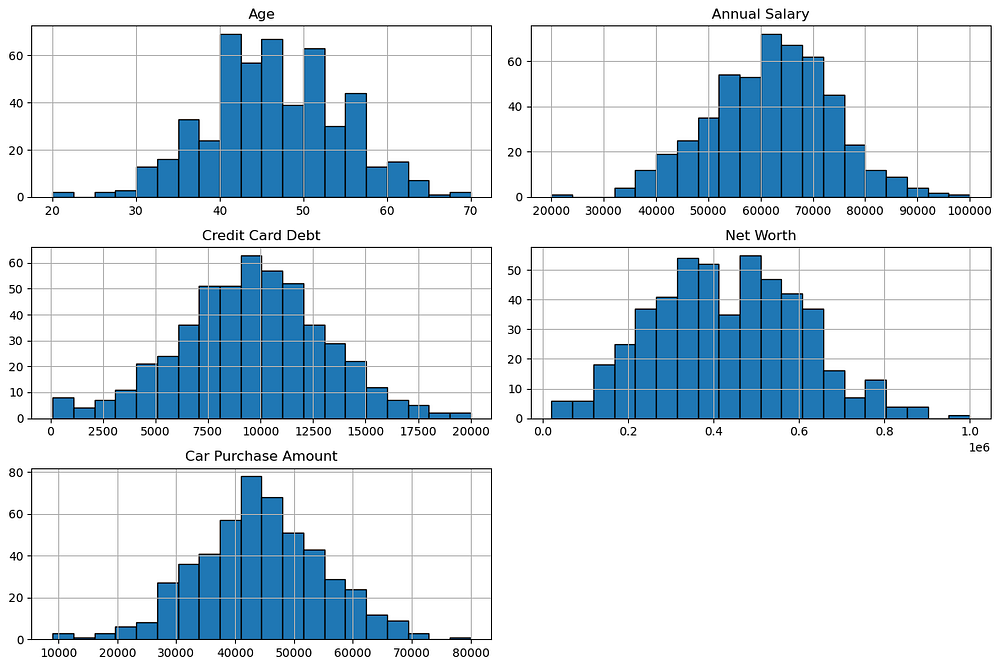
# Plot histograms for numerical features
data[['Age', 'Annual Salary', 'Credit Card Debt', 'Net Worth', 'Car Purchase Amount']].hist(
    figsize=(12, 8), bins=20, edgecolor='black')
plt.tight_layout()
plt.show()

This plot provides the following insights:

Age: The age distribution is approximately normal, with most customers aged between 40 and 50.
Annual Salary: Salaries are normally distributed, peaking around $60,000 to $70,000.
Credit Card Debt: Debt levels are normally distributed, centred near $10,000.
Net Worth: Net worth is slightly right-skewed, with most values concentrated between $300,000 and $600,000.
Car Purchase Amount: The target variable follows a roughly normal distribution, peaking around $40,000 to $50,000.

These distributions suggest balanced data for modelling, with no major irregularities or extreme skewness.

Correlation Analysis

To identify relationships between numerical features:

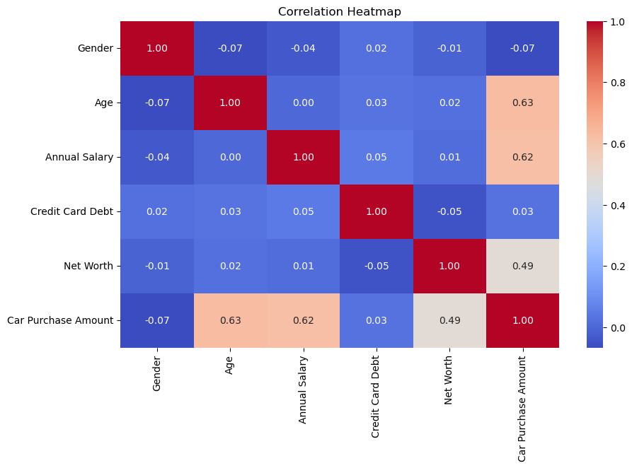
# Plot a correlation heatmap
plt.figure(figsize=(10, 6))
sns.heatmap(data.corr(), annot=True, cmap='coolwarm', fmt='.2f')
plt.title('Correlation Heatmap')
plt.show()

This correlation heatmap reveals the following insights:

Age and Annual Salary both have strong positive correlations with Car Purchase Amount (0.63 and 0.62, respectively), making them important predictors.
Net Worth has a moderate positive correlation with Car Purchase Amount (0.49), suggesting it is also a relevant feature.
Other features like Gender and Credit Card Debt have very weak or negligible correlations with Car Purchase Amount, indicating they may contribute less to the prediction.

Overall, financial metrics and age are the most influential factors for predicting car purchase amounts.

Pair Plot

To visualize pairwise relationships:

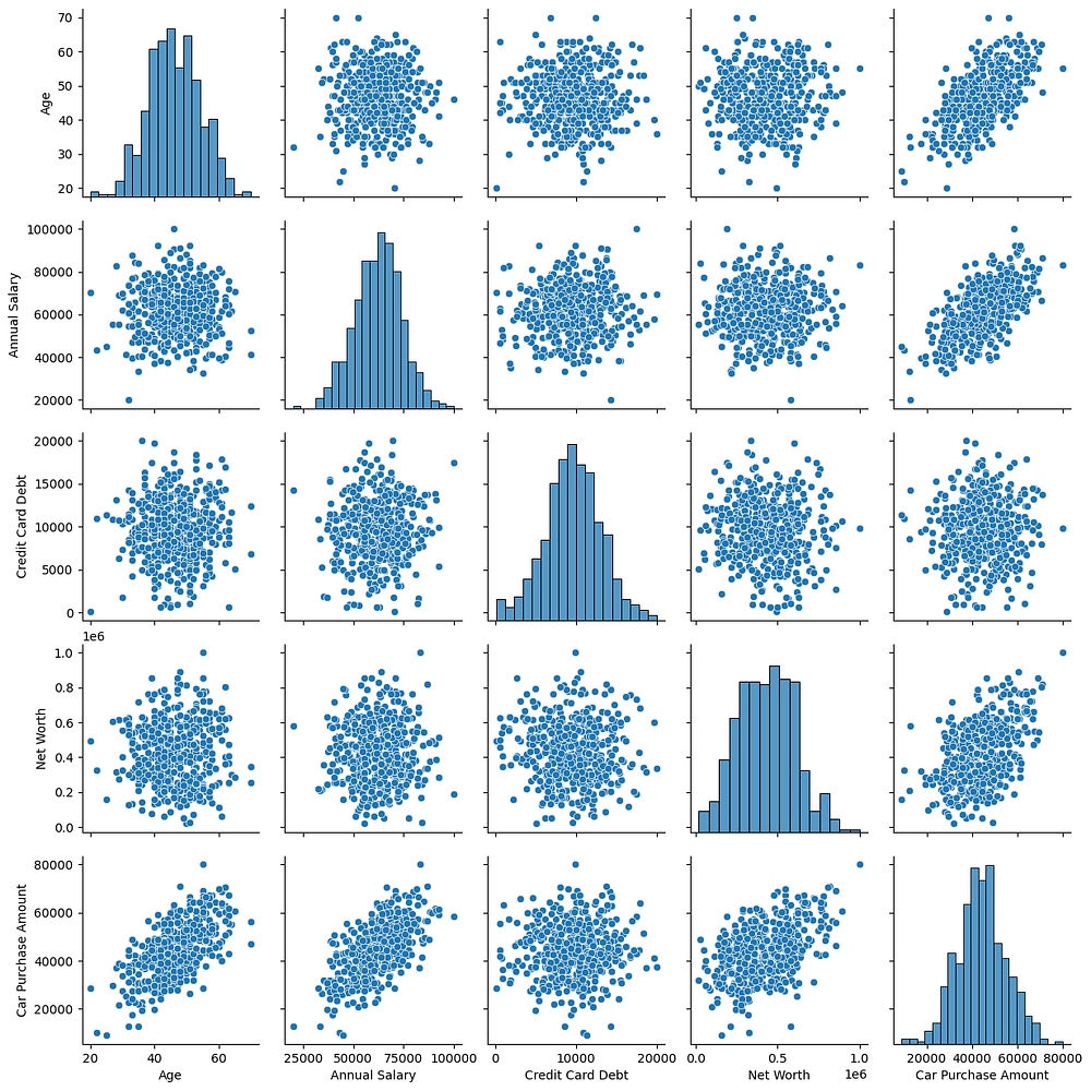
# Generate a pair plot
sns.pairplot(data[['Age', 'Annual Salary', 'Credit Card Debt', 'Net Worth', 'Car Purchase Amount']])
plt.show()

This pair plot provides the following insights:

Age, Annual Salary, and Net Worth show positive linear relationships with Car Purchase Amount, confirming their predictive relevance.
Credit Card Debt does not show a clear relationship with Car Purchase Amount, indicating it may have less predictive value.
Features like Annual Salary and Net Worth show strong positive correlations with each other, which could lead to multicollinearity.
All numerical features exhibit fairly normal distributions, suitable for regression modelling.

This visualization supports the importance of key financial metrics in predicting Car Purchase Amount.

4. Data Preparation and Feature Engineering

Before building the model, we need to clean and prepare the data to ensure it is suitable for training. This involves handling missing values, scaling numerical features, and selecting relevant features.

Handling Missing Values

We check for and address any missing values in the dataset:

# Check for missing values
print(data.isnull().sum())

Customer Name          0
Customer e-mail        0
Country                0
Gender                 0
Age                    0
Annual Salary          0
Credit Card Debt       0
Net Worth              0
Car Purchase Amount    0
dtype: int64

The dataset does not have missing values, so no further action is needed.

Feature Selection

We drop irrelevant columns that do not contribute to prediction, such as Customer Name, Customer e-mail, and Country.

# Drop irrelevant columns
data = data.drop(['Customer Name', 'Customer e-mail', 'Country'], axis=1)

Encoding Categorical Variables

The Gender column is already encoded as numerical values (0 for male, 1 for female), so no further encoding is required.

Scaling Numerical Features

To ensure all features are on the same scale, we use StandardScaler:

from sklearn.preprocessing import StandardScaler

# Separate features and target variable
X = data.drop('Car Purchase Amount', axis=1)  # Features
y = data['Car Purchase Amount']  # Target variable

# Apply scaling
scaler = StandardScaler()
X_scaled = scaler.fit_transform(X)

Scaling is crucial because features like Net Worth and Credit Card Debt are on different scales, which could bias the model.

5. Model Building and Evaluation

To streamline the model selection and evaluation process, we will use an AutoML package to automatically train, evaluate, and fine-tune a range of regression models. This approach ensures that we identify the best-performing model without manually testing each algorithm.

Installing and Importing AutoML Package

We use the PyCaret library for AutoML. If it's not already installed, you can install it as follows:

pip install pycaret

Import the required modules:

from pycaret.regression import setup, compare_models, pull, save_model

Initializing the AutoML Environment

We initialize the AutoML pipeline using setup() to specify the dataset, target variable, and configuration options:

# Initialize PyCaret regression setup
automl = setup(
    data=data,
    target='Car Purchase Amount',  # Target variable
    train_size=0.8,                # Train-test split ratio
    session_id=42,                 # For reproducibility
    normalize=True                 # Ensures feature scaling
)

Key Parameters:

data: The dataset.
target: The column to predict (Car Purchase Amount).
normalize: Automatically scales numerical features for better model performance.

Training and Selecting the Best Model

We use compare_models() to test multiple regression models and select the best one based on performance metrics such as Mean Absolute Error (MAE):

# Compare models and select the best one
best_model = compare_models(sort='MAE')

The compare_models() function evaluates a range of regression models, such as:

Linear Regression
Ridge Regression
Random Forest
Gradient Boosting
Neural Networks

It ranks models based on the chosen metric (MAE in this case).

Viewing Model Results

We can view the detailed results of all tested models using the pull() function:

# Display comparison results
results = pull()
print(results)

                                    Model        MAE           MSE  \
par          Passive Aggressive Regressor   208.0755  5.976193e+04   
br                         Bayesian Ridge   208.7050  5.860764e+04   
lar                Least Angle Regression   208.7060  5.860718e+04   
lr                      Linear Regression   208.7063  5.860726e+04   
huber                     Huber Regressor   208.7345  5.924132e+04   
llar         Lasso Least Angle Regression   208.7610  5.862013e+04   
lasso                    Lasso Regression   208.7614  5.862036e+04   
ridge                    Ridge Regression   208.7838  5.955234e+04   
catboost               CatBoost Regressor   759.9736  2.431932e+06   
et                  Extra Trees Regressor  1230.1609  4.432660e+06   
gbr           Gradient Boosting Regressor  1353.6206  3.992229e+06   
lightgbm  Light Gradient Boosting Machine  1385.5471  4.846046e+06   
xgboost         Extreme Gradient Boosting  1585.8605  5.859166e+06   
rf                Random Forest Regressor  1796.2792  7.348954e+06   
knn                 K Neighbors Regressor  2748.0798  1.436356e+07   
en                            Elastic Net  2833.3671  1.310012e+07   
ada                    AdaBoost Regressor  3169.2546  1.869494e+07   
dt                Decision Tree Regressor  3244.9663  1.971123e+07   
omp           Orthogonal Matching Pursuit  7118.7649  7.960319e+07   
dummy                     Dummy Regressor  8492.6023  1.179679e+08   

                RMSE      R2   RMSLE    MAPE  TT (Sec)  
par         243.5812  0.9994  0.0062  0.0051     0.012  
br          241.3427  0.9995  0.0062  0.0051     0.006  
lar         241.3415  0.9995  0.0062  0.0051     0.007  
lr          241.3417  0.9995  0.0062  0.0051     0.814  
huber       242.6528  0.9994  0.0062  0.0051     0.007  
llar        241.3800  0.9995  0.0062  0.0051     0.008  
lasso       241.3805  0.9995  0.0062  0.0051     0.521  
ridge       243.3959  0.9994  0.0062  0.0051     0.013  
catboost   1441.0213  0.9804  0.0507  0.0242     0.457  
et         2023.9017  0.9626  0.0712  0.0383     0.023  
gbr        1970.8825  0.9653  0.0648  0.0381     0.016  
lightgbm   2127.9460  0.9589  0.0710  0.0408     0.047  
xgboost    2253.0673  0.8504  0.0743  0.0458     0.154  
rf         2638.4407  0.9382  0.0855  0.0523     0.027  
knn        3759.1558  0.8749  0.1130  0.0766     0.011  
en         3599.7438  0.8860  0.1072  0.0776     0.006  
ada        4277.6572  0.8386  0.1275  0.0887     0.020  
dt         4358.9889  0.8303  0.1271  0.0861     0.007  
omp        8896.6669  0.2925  0.2295  0.1892     0.007  
dummy     10809.2149 -0.0295  0.2766  0.2327     0.006

This result summarizes the performance of various regression models tested using an AutoML package. Key observations:

Top Performers: Passive Aggressive Regressor, Bayesian Ridge, Least Angle Regression, and Linear Regression have the lowest MAE (~208) and RMSE (~241), with the highest R² (~0.9995), making them the most suitable models for this dataset.
Underperformers: Dummy Regressor and Orthogonal Matching Pursuit performed poorly, with very high MAE (>7,000) and negative/low R² values, indicating they fail to explain the variance in the data.
Tree-Based Models: Models like CatBoost Regressor, Extra Trees Regressor, and Gradient Boosting Regressor showed decent performance (R² ~0.96–0.98) but significantly higher errors (MAE > 750), making them less competitive.
Neural Networks and Ensembles: Models like LightGBM and AdaBoost Regressor have moderate R² (0.83–0.96) but considerably higher MAE and RMSE.
Efficiency: Top-performing models (e.g., Bayesian Ridge, Linear Regression) trained quickly (<1 second), making them both effective and computationally efficient.

For this dataset, Passive Aggressive Regressor*,* Bayesian Ridge*, and* Linear Regression are the top-performing models. They exhibit:

High Accuracy*: Low MAE (~208) and RMSE (~241), with R² values close to 1.*
Efficiency*: Very fast training times (all under 1 second).*
Simplicity*: These models do not require complex feature engineering or additional computation, making them practical for deployment.*

While more complex models (e.g., CatBoost, Gradient Boosting) also perform well, their higher error rates and computational cost make them less suitable for this project. The Passive Aggressive Regressor should be included as a strong candidate.

7. Deployment with Streamlit

To make the trained model accessible for real-world use, we will deploy it using Streamlit, a Python framework for building interactive web apps. Based on our evaluation, the Passive Aggressive Regressor was selected as the best model for deployment due to its high accuracy, low error, and fast training time. The deployment process involves saving this trained model using joblib, creating a Streamlit app, and enabling users to input data and receive predictions.

Step 1: Save the Trained Model

We use joblib to save the best-performing model for later use in the Streamlit app:

# Save the scaler
joblib.dump(scaler, 'scaler.pkl')
print("Scaler saved as 'scaler.pkl'")

# Save the trained model
joblib.dump(best_model, 'car_purchase_model.pkl')
print("Model saved as 'car_purchase_model.pkl'")

Scaler saved as 'scaler.pkl'
Model saved as 'car_purchase_model.pkl'

Step 2: Create the Streamlit App

We create an app.py file to build the interactive app:

import streamlit as st
import joblib
import numpy as np
from sklearn.preprocessing import StandardScaler

# Load the saved model and scaler
model = joblib.load('car_purchase_model.pkl')
scaler = joblib.load('scaler.pkl')  # Save and load the scaler used during training

# Define the app interface
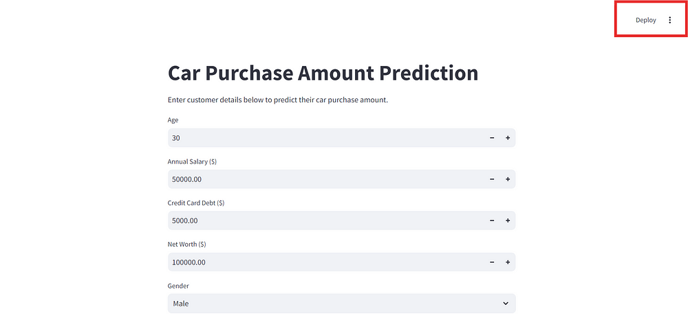
st.title("Car Purchase Amount Prediction")
st.write("Enter customer details below to predict their car purchase amount.")

# Input fields for user data
age = st.number_input("Age", min_value=18, max_value=100, step=1, value=30)
annual_salary = st.number_input("Annual Salary ($)", min_value=0.0, step=1000.0, value=50000.0)
credit_card_debt = st.number_input("Credit Card Debt ($)", min_value=0.0, step=100.0, value=5000.0)
net_worth = st.number_input("Net Worth ($)", min_value=0.0, step=1000.0, value=100000.0)
gender = st.selectbox("Gender", options=["Male", "Female"])

# Encode gender as numerical value
gender_encoded = 0 if gender == "Male" else 1

# Predict button
if st.button("Predict"):
    # Prepare input data as a NumPy array
    input_data = np.array([[gender_encoded, age, annual_salary, credit_card_debt, net_worth]])

    # Apply the same scaling as during training
    input_data_scaled = scaler.transform(input_data)

    # Make prediction
    prediction = model.predict(input_data_scaled)

    # Display the result
    st.success(f"Predicted Car Purchase Amount: ${prediction[0]:,.2f}")

Step 3: Run the Streamlit App

To run the app locally, use the following command in your terminal:
Build a simple Streamlit app for practical model deployment.

streamlit run streamlit_app.py

Step 4: Generate a `requirements.txt` file

The requirements.txt file is essential for the model to be deployed on Streamlit Cloud, it will tell which modules need to be imported to run the model:

streamlit
joblib
numpy
pandas
scikit-learn

Step 5: Deploy the Streamlit App on the Streamlit Cloud Community (optional)

You can click on the Deploy button on the top right of the app interface (after pushing the repo to Github), and then the app will be deployed after a few seconds.

The result will look like this:

https://minhhoang2606-car-price-prediction-by-machine-learni-app-65yvev.streamlit.app/

8. Conclusion

In this project, we developed a machine learning model to predict Car Purchase Amounts based on customer demographic and financial data. The Passive Aggressive Regressor was selected as the best-performing model due to its high accuracy, low error, and fast training time. Using Streamlit, we deployed the model to create an interactive app that allows users to input customer details and receive real-time purchase predictions.

Through this process, we demonstrated the importance of:

Exploratory Data Analysis: Understanding data distributions and relationships to identify meaningful patterns.
Automated Model Selection: Leveraging tools like AutoML to efficiently compare and optimize models.
Deployment: Making machine learning solutions accessible to end-users through simple and intuitive interfaces.

This project highlights how machine learning can empower businesses by providing actionable insights, improving decision-making, and enhancing customer experiences. The deployed app can be further extended for real-world use, such as integrating additional features, handling larger datasets, or deploying on cloud platforms for scalability.

Appendices

Code: https://github.com/Minhhoang2606/Car-Purchase-Amount-Predictions-Using-Machine-Learning

Data source: https://www.kaggle.com/datasets/dev0914sharma/car-purchasing-model?select=Car_Purchasing_Data.csv

Car Purchase Amount Predictions Using Machine Learning

Table of contents

1. Introduction

2. Dataset Overview

3. Exploratory Data Analysis (EDA)

Dataset Snapshot

Descriptive Statistics

Feature Distributions

Correlation Analysis

Pair Plot

4. Data Preparation and Feature Engineering

Handling Missing Values

Feature Selection

Encoding Categorical Variables

Scaling Numerical Features

5. Model Building and Evaluation

Installing and Importing AutoML Package

Initializing the AutoML Environment

Training and Selecting the Best Model

Viewing Model Results

7. Deployment with Streamlit

Step 1: Save the Trained Model

Step 2: Create the Streamlit App

Step 3: Run the Streamlit App

Step 4: Generate a `requirements.txt` file

Step 5: Deploy the Streamlit App on the Streamlit Cloud Community (optional)

8. Conclusion

Appendices

Car Purchase Amount Predictions Using Machine Learning

Table of contents

1. Introduction

2. Dataset Overview

3. Exploratory Data Analysis (EDA)

Dataset Snapshot

Descriptive Statistics

Feature Distributions

Correlation Analysis

Pair Plot

4. Data Preparation and Feature Engineering

Handling Missing Values

Feature Selection

Encoding Categorical Variables

Scaling Numerical Features

5. Model Building and Evaluation

Installing and Importing AutoML Package

Initializing the AutoML Environment

Training and Selecting the Best Model

Viewing Model Results

7. Deployment with Streamlit

Step 1: Save the Trained Model

Step 2: Create the Streamlit App

Step 3: Run the Streamlit App

Step 4: Generate a requirements.txt file

Step 5: Deploy the Streamlit App on the Streamlit Cloud Community (optional)

8. Conclusion

Appendices

Step 4: Generate a `requirements.txt` file