1. Introduction

The avocado market has gained significant attention in recent years, with its price trends often reflecting shifts in consumer demand, supply chain dynamics, and even cultural preferences. Predicting avocado prices can offer valuable insights for stakeholders such as farmers, retailers, and policymakers. By leveraging machine learning, we can analyze historical data to build predictive models that forecast future price fluctuations, enabling better decision-making and strategic planning.

This project focuses on building a robust machine learning pipeline to predict avocado prices. We will explore the dataset, perform detailed exploratory data analysis (EDA), preprocess the data, and evaluate multiple regression models to identify the best approach. The insights gained can help optimize inventory management, pricing strategies, and market supply.

2. Understanding the Dataset

The dataset used in this project contains information about avocado sales and pricing across various regions in the United States over multiple years. Each row represents a specific observation of avocado sales, including details such as the type of avocado (conventional or organic), volume sold, and average price. Below is a summary of the key features:

Date: The date of the observation.
AveragePrice (target variable): The average price of a single avocado.
Total Volume: The total number of avocados sold.
4046, 4225, 4770: Sales volume of different sizes of avocados.
Total Bags: The total number of bags sold.
Small Bags, Large Bags, XLarge Bags: Breakdown of bag sizes sold.
Type: The type of avocado (Conventional or Organic).
Year: The year of the observation.
Region: The geographical region of the sales.

Initial Observations

The dataset spans multiple years and includes both conventional and organic avocados, allowing comparative analysis.
Features such as sales volume and bag size categories provide granular insights into consumption patterns.
The “Region” column includes numerous unique values, making it a candidate for encoding or aggregation to reduce complexity.
The target variable, AveragePrice, is continuous, making this a regression problem.

Understanding this dataset’s structure and nuances is critical as it will guide our exploratory data analysis and model-building process. In the next steps, we will delve deeper into visualizing and preparing the data for effective modelling.

3. Exploratory Data Analysis (EDA)

Exploratory Data Analysis (EDA) is a critical step in understanding the dataset, uncovering patterns, and identifying potential challenges. Through visualizations and statistical analysis, we can gain insights into the relationships between features and the target variable.

Importing the Data and General Information

We start by loading the dataset and inspecting its structure to identify any missing values or anomalies.

import pandas as pd

# Load the dataset
df = pd.read_csv('avocado.csv')
# Display the first few rows
print(df.head())
# Display general information about the dataset
print(df.info())
# Summary statistics for numerical features
print(df.describe())

   Unnamed: 0        Date  AveragePrice  Total Volume     4046       4225  \
0           0  2015-12-27          1.33      64236.62  1036.74   54454.85   
1           1  2015-12-20          1.35      54876.98   674.28   44638.81   
2           2  2015-12-13          0.93     118220.22   794.70  109149.67   
3           3  2015-12-06          1.08      78992.15  1132.00   71976.41   
4           4  2015-11-29          1.28      51039.60   941.48   43838.39   

     4770  Total Bags  Small Bags  Large Bags  XLarge Bags          type  \
0   48.16     8696.87     8603.62       93.25          0.0  conventional   
1   58.33     9505.56     9408.07       97.49          0.0  conventional   
2  130.50     8145.35     8042.21      103.14          0.0  conventional   
3   72.58     5811.16     5677.40      133.76          0.0  conventional   
4   75.78     6183.95     5986.26      197.69          0.0  conventional   

   year  region  
0  2015  Albany  
1  2015  Albany  
2  2015  Albany  
3  2015  Albany  
4  2015  Albany  
<class 'pandas.core.frame.DataFrame'>
RangeIndex: 18249 entries, 0 to 18248
Data columns (total 14 columns):
 #   Column        Non-Null Count  Dtype  
---  ------        --------------  -----  
 0   Unnamed: 0    18249 non-null  int64  
 1   Date          18249 non-null  object 
 2   AveragePrice  18249 non-null  float64
 3   Total Volume  18249 non-null  float64
 4   4046          18249 non-null  float64
 5   4225          18249 non-null  float64
 6   4770          18249 non-null  float64
 7   Total Bags    18249 non-null  float64
 8   Small Bags    18249 non-null  float64
 9   Large Bags    18249 non-null  float64
 10  XLarge Bags   18249 non-null  float64
 11  type          18249 non-null  object 
 12  year          18249 non-null  int64  
 13  region        18249 non-null  object 
dtypes: float64(9), int64(2), object(3)
memory usage: 1.9+ MB
None
         Unnamed: 0  AveragePrice  Total Volume          4046          4225  \
count  18249.000000  18249.000000  1.824900e+04  1.824900e+04  1.824900e+04   
mean      24.232232      1.405978  8.506440e+05  2.930084e+05  2.951546e+05   
std       15.481045      0.402677  3.453545e+06  1.264989e+06  1.204120e+06   
min        0.000000      0.440000  8.456000e+01  0.000000e+00  0.000000e+00   
25%       10.000000      1.100000  1.083858e+04  8.540700e+02  3.008780e+03   
50%       24.000000      1.370000  1.073768e+05  8.645300e+03  2.906102e+04   
75%       38.000000      1.660000  4.329623e+05  1.110202e+05  1.502069e+05   
max       52.000000      3.250000  6.250565e+07  2.274362e+07  2.047057e+07   

               4770    Total Bags    Small Bags    Large Bags    XLarge Bags  \
count  1.824900e+04  1.824900e+04  1.824900e+04  1.824900e+04   18249.000000   
mean   2.283974e+04  2.396392e+05  1.821947e+05  5.433809e+04    3106.426507   
std    1.074641e+05  9.862424e+05  7.461785e+05  2.439660e+05   17692.894652   
min    0.000000e+00  0.000000e+00  0.000000e+00  0.000000e+00       0.000000   
25%    0.000000e+00  5.088640e+03  2.849420e+03  1.274700e+02       0.000000   
50%    1.849900e+02  3.974383e+04  2.636282e+04  2.647710e+03       0.000000   
75%    6.243420e+03  1.107834e+05  8.333767e+04  2.202925e+04     132.500000   
max    2.546439e+06  1.937313e+07  1.338459e+07  5.719097e+06  551693.650000   

               year  
count  18249.000000  
mean    2016.147899  
std        0.939938  
min     2015.000000  
25%     2015.000000  
50%     2016.000000  
75%     2017.000000  
max     2018.000000  
<ipython-input-4-2a52aa0a99ea>:25: FutureWarning: The default value of numeric_only in DataFrameGroupBy.mean is deprecated. In a future version, numeric_only will default to False. Either specify numeric_only or select only columns which should be valid for the function.
  df_grouped = df.groupby('Date').mean()

Dataset Overview:

The dataset contains 14 columns and 18,249 rows with no missing values. Key features include sales data (e.g., Total Volume, 4046, 4225) and categorical variables such as type and region.
Target variable: AveragePrice (continuous).

2. Data Types:

Numerical features dominate the dataset (e.g., AveragePrice, Total Volume), making it suitable for regression analysis.
type and region are categorical and require encoding.

3. Summary Statistics:

Price Range: AveragePrice varies between $0.44 and $3.25, with a mean of $1.41.
Sales Volume: A wide range of sales volumes, with Total Volume reaching up to 62.5 million, highlights market variability.
Bag Sizes: Most bags sold are small, with larger bags being far less common (XLarge Bags mean is 3,106 compared to Small Bags mean of 182,194).

4. Year Distribution:

Data spans from 2015 to 2018, providing multiple years for temporal trend analysis.

These insights guide the EDA to explore relationships between features, temporal patterns, and regional price variations. Let me know if you’d like further elaboration or adjustments!

Price Trends Over Time

import matplotlib.pyplot as plt

df['Date'] = pd.to_datetime(df['Date'])
df_grouped = df.groupby('Date').mean()

plt.figure(figsize=(12, 6))
plt.plot(df_grouped.index, df_grouped['AveragePrice'], label='Average Price')
plt.title('Average Avocado Price Over Time')
plt.xlabel('Date')
plt.ylabel('Average Price')
plt.legend()
plt.show()

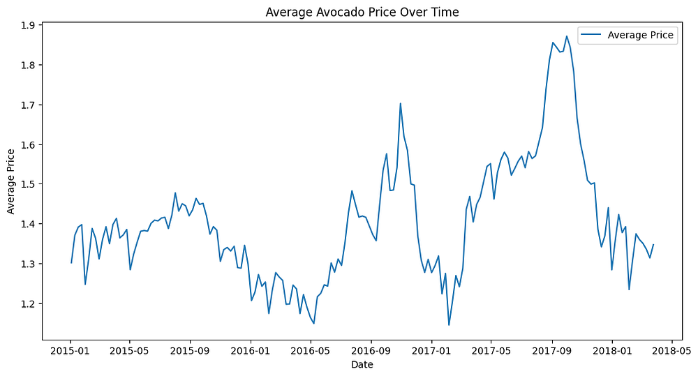
General Trend:
- The average avocado price shows significant fluctuations between 2015 and 2018.
- A clear upward trend is observed from mid-2016, peaking around mid-2017, followed by a gradual decline.
Seasonal Patterns: Prices tend to have periodic spikes, suggesting seasonal demand or supply variations.
Price Peaks: The highest price levels occurred around mid-2017, possibly due to market constraints or increased demand.
Implications: This trend highlights the importance of accounting for time-based variations in pricing and the potential impact of external factors like supply chain disruptions or consumer trends.

Price by Type

import seaborn as sns

plt.figure(figsize=(8, 6))
sns.boxplot(x='type', y='AveragePrice', data=df)
plt.title('Price Distribution by Type')
plt.xlabel('Type')
plt.ylabel('Average Price')
plt.show()

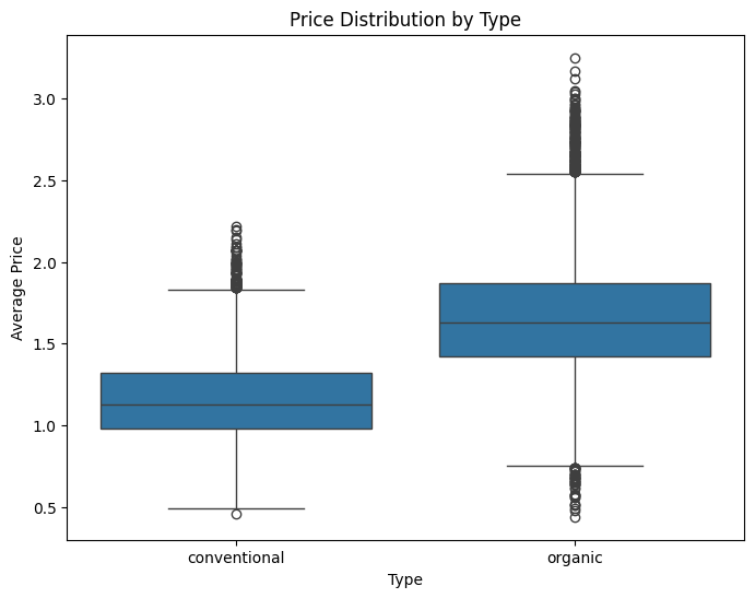
Price Comparison:

Organic avocados consistently have a higher median price compared to conventional ones.
This reflects the premium pricing often associated with organic products.

2. Price Distribution:

Conventional avocados exhibit a narrower interquartile range (IQR), indicating more consistent pricing.
Organic avocados have a wider IQR and more outliers, suggesting greater price variability.

3. Implications:

The price difference highlights the need to treat type as an essential feature in predictive modelling.
The variability in organic prices might be influenced by regional or seasonal factors.

Sales Volume and Price Correlation

plt.figure(figsize=(8, 6))
sns.scatterplot(x='Total Volume', y='AveragePrice', data=df)
plt.title('Total Volume vs. Average Price')
plt.xlabel('Total Volume')
plt.ylabel('Average Price')
plt.show()

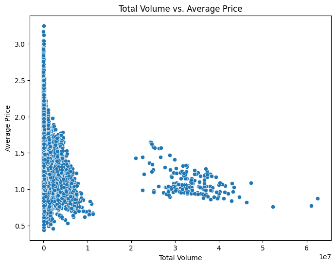
Relationship: There is a clear negative correlation between total volume and average price. As the total volume increases, the average price tends to decrease.
Market Dynamics: The trend suggests a supply-demand relationship: higher supply leads to lower prices. This is typical for commodities like avocados.
Clusters: Two distinct clusters are visible: One with a high price and low volume and another with a moderate price and higher volume.
Implications: Pricing strategies should consider supply levels. Besides, the clustering suggests differences in market conditions, possibly influenced by regional or temporal factors.

Regional Price Analysis

regional_avg_price = df.groupby('region')['AveragePrice'].mean().sort_values()

plt.figure(figsize=(12, 8))
regional_avg_price.plot(kind='bar', color='skyblue')
plt.title('Average Price by Region')
plt.xlabel('Region')
plt.ylabel('Average Price')
plt.xticks(rotation=90)
plt.show()

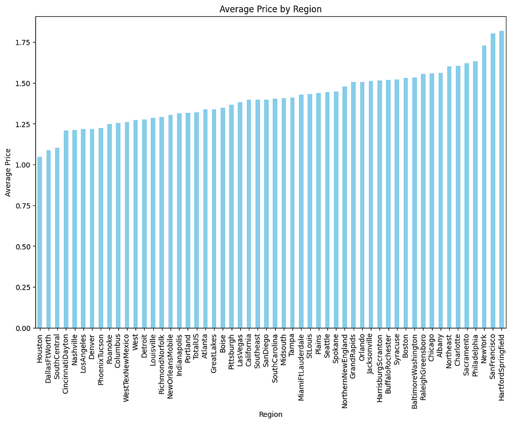
Regional Price Variations:

Significant differences in average avocado prices are observed across regions.
Regions like Hartford/Springfield have the highest average prices, while Houston and Dallas/Fort Worth have the lowest.

2. Implications:

Regional price disparities may reflect variations in supply chains, demand, or local market conditions.
High-price regions could indicate limited supply or higher consumer willingness to pay for avocados.

3. Actionable Insights:

Pricing models should account for regional factors.
Further analysis could explore correlations with demographic or economic data for deeper insights.

Checking Linear Regression Conditions (Basic Checks)

As part of the EDA, we perform basic checks to assess whether the data aligns with the conditions required for Linear Regression. This step focuses on identifying potential issues early, such as linearity and multicollinearity, which could influence model performance. Firstly, we will check the linearity:

Purpose: Ensure there is a linear relationship between the independent variables and the target variable (AveragePrice).
How to Check: Use scatterplots to visually inspect the relationship.

# Scatterplots for linearity check
sns.pairplot(df, y_vars='AveragePrice', x_vars=['Total Volume', '4046', '4225', '4770'])
plt.show()

The scatterplots show a clear non-linear relationship between AveragePrice and the independent variables (Total Volume, 4046, 4225, 4770). As the values of these variables increase, AveragePrice tends to decrease, indicating a negative correlation. However, the funnel-shaped spread suggests heteroscedasticity, meaning the variance of AveragePrice is not constant across all levels of the predictors. This indicates a potential need for transformations (e.g., log transformation) to meet the linearity assumption for Linear Regression. The next part will check the multicollinearity of the features.

Correlation Heatmap

plt.figure(figsize=(10, 6))
correlation = df.corr()
sns.heatmap(correlation, annot=True, cmap='coolwarm', fmt='.2f')
plt.title('Correlation Heatmap')
plt.show()

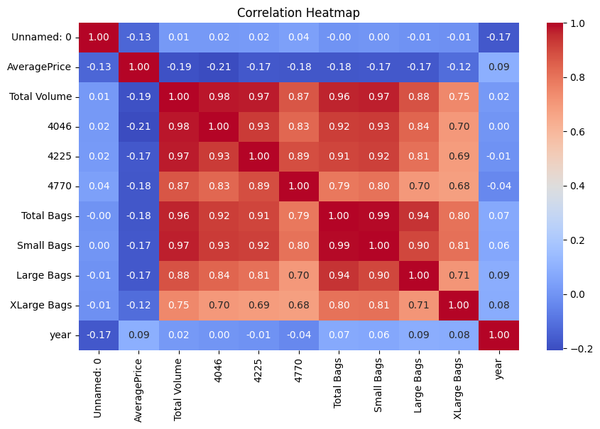
Strong Positive Correlations:

Total Volume has high correlations with 4046, 4225, and Total Bags (above 0.95). This suggests that these features collectively influence the total volume significantly.
Small Bags and Total Bags are almost perfectly correlated (0.99), indicating redundancy.

2. Negative Correlation with AveragePrice: AveragePrice shows weak negative correlations with Total Volume (-0.19) and related features (4046, 4225, etc.). This supports the inverse relationship between supply and price.

3. Insights for Feature Engineering: Features with extremely high correlations, such as Small Bags and Total Bags, might be considered for removal or consolidation to avoid multicollinearity.

4. Data Preprocessing

Data preprocessing is a crucial step to ensure the dataset is clean, consistent, and ready for machine learning models. This involves handling missing values, encoding categorical features, and standardizing the data.

Handling Missing Values

Since the dataset does not contain missing values (info() confirmed), no imputation is needed.

Encoding Categorical Variables

The type and region columns are categorical and need to be encoded.

# One-hot encoding for the 'type' and 'region' columns 
df = pd.get_dummies(df, columns=['type', 'region'], drop_first=True)

Feature Engineering

Drop unnecessary columns, such as Unnamed: 0, which is just an index column.

df = df.drop(columns=['Unnamed: 0'])

Extract temporal information from the Date column for potential seasonality patterns.

df['month'] = df['Date'].dt.month
df['day'] = df['Date'].dt.day

Splitting the Dataset

Separate the features and the target variable (AveragePrice).

X = df.drop(columns=['AveragePrice', 'Date'])
y = df['AveragePrice']

Scaling Numerical Features

Standardize the numerical features to improve model performance.

from sklearn.preprocessing import StandardScaler

scaler = StandardScaler()
X_scaled = scaler.fit_transform(X)

Full Assessment of Linear Regression Conditions

After completing the data preprocessing, we perform a full assessment to ensure that the final dataset meets the key assumptions required for Linear Regression. These checks include residual analysis, homoscedasticity, and normality to validate the model’s suitability.

Independence of Errors

Purpose: Ensure that the residuals (errors) are independent.
How to Check: Use the Durbin-Watson statistic to test for autocorrelation.

from statsmodels.stats.stattools import durbin_watson

# Calculate residuals
residuals = y_test - lr_model.predict(X_test)

# Durbin-Watson test
print("Durbin-Watson Statistic:", durbin_watson(residuals))

Homoscedasticity Check

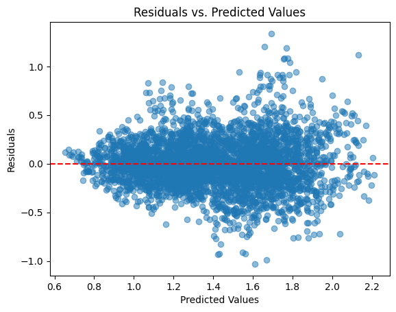
Purpose: Verify that the variance of residuals remains constant across predicted values.
How to Check: Plot residuals vs. predicted values.

# Homoscedasticity Check
plt.scatter(lr_model.predict(X_test), residuals, alpha=0.5)
plt.axhline(y=0, color='red', linestyle='--')
plt.title("Residuals vs. Predicted Values")
plt.xlabel("Predicted Values")
plt.ylabel("Residuals")
plt.show()

The residuals vs. predicted values plot shows that the residuals are randomly scattered around the horizontal line at 0, indicating no clear pattern. This suggests that the assumption of homoscedasticity (constant variance of residuals) is met, and there is no evidence of systematic bias in the predictions. The model appears to be appropriate in terms of this condition.

These steps ensure the dataset is clean and optimized for model training. In the next section, we will build and evaluate regression models to predict avocado prices.

5. Model Building

In this section, we will train three regression models to predict avocado prices: Linear Regression, Decision Tree Regressor, and Random Forest Regressor. These models are chosen for their simplicity, interpretability, and ability to capture complex patterns.

Linear Regression

from sklearn.linear_model import LinearRegression
from sklearn.model_selection import train_test_split

# Split the data
X_train, X_test, y_train, y_test = train_test_split(X_scaled, y, test_size=0.2, random_state=42)

# Train the model
lr_model = LinearRegression()
lr_model.fit(X_train, y_train)

Decision Tree Regressor

from sklearn.tree import DecisionTreeRegressor

# Train the model
dt_model = DecisionTreeRegressor(random_state=42)
dt_model.fit(X_train, y_train)

Random Forest Regressor

from sklearn.ensemble import RandomForestRegressor

# Train the model
rf_model = RandomForestRegressor(n_estimators=100, random_state=42)
rf_model.fit(X_train, y_train)

6. Model Evaluation

Evaluating the performance of the models is essential to determine their predictive capabilities. We use metrics such as Mean Absolute Error (MAE), Mean Squared Error (MSE), and R-squared (R²) to compare the performance of Linear Regression, Decision Tree Regressor, and Random Forest Regressor.

Linear Regression

# Linear Regression
from sklearn.metrics import mean_absolute_error, mean_squared_error, r2_score

# Predictions
y_pred_lr = lr_model.predict(X_test)

# Metrics
print("Linear Regression:")
print("MAE:", mean_absolute_error(y_test, y_pred_lr))
print("MSE:", mean_squared_error(y_test, y_pred_lr))
print("R²:", r2_score(y_test, y_pred_lr))

# Visualization of predicted prices vs. actual prices of the linear regression model
plt.figure(figsize=(8, 6))
plt.scatter(y_test, y_pred_lr, alpha=0.5)
plt.plot([y_test.min(), y_test.max()], [y_test.min(), y_test.max()], color='red', linestyle='--', linewidth=2)
plt.title("Linear Regression: Predictions vs. Actual Prices")
plt.xlabel("Actual Prices")
plt.ylabel("Predicted Prices")
plt.show()

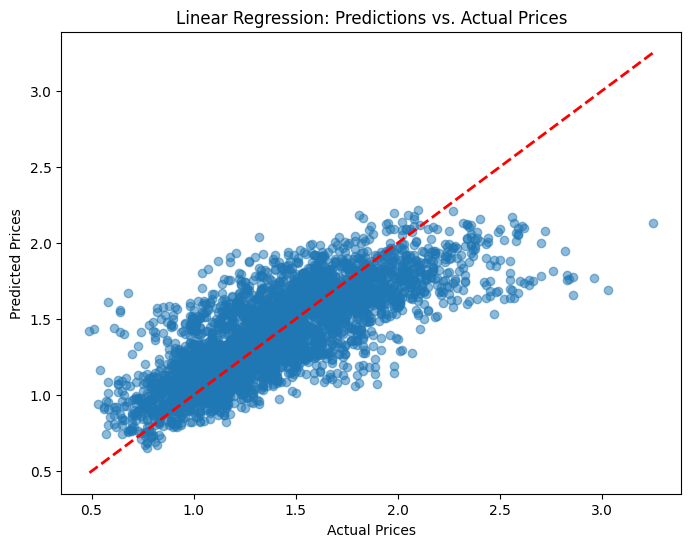
Linear Regression:
MAE: 0.19464779933226573
MSE: 0.06622078348044358
R²: 0.5878436466242649

Decision Tree Regressor

# Decision Tree Regressor
# Predictions
y_pred_dt = dt_model.predict(X_test)

# Metrics
print("Decision Tree Regressor:")
print("MAE:", mean_absolute_error(y_test, y_pred_dt))
print("MSE:", mean_squared_error(y_test, y_pred_dt))
print("R²:", r2_score(y_test, y_pred_dt))

# Visualization of predicted prices vs. actual prices of the decision tree regressor model
plt.figure(figsize=(8, 6))
plt.scatter(y_test, y_pred_dt, alpha=0.5, color='green')
plt.plot([y_test.min(), y_test.max()], [y_test.min(), y_test.max()], color='red', linestyle='--', linewidth=2)
plt.title("Decision Tree: Predictions vs. Actual Prices")
plt.xlabel("Actual Prices")
plt.ylabel("Predicted Prices")
plt.show()

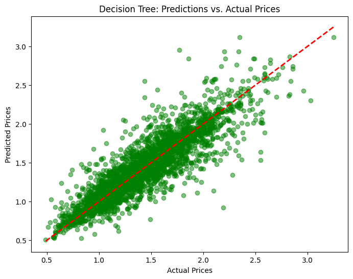
Decision Tree Regressor:
MAE: 0.12177808219178082
MSE: 0.03348090410958904
R²: 0.7916157644132052

Random Forest Regressor

# Random Forest Regressor

# Predictions
y_pred_rf = rf_model.predict(X_test)

# Metrics
print("Random Forest Regressor:")
print("MAE:", mean_absolute_error(y_test, y_pred_rf))
print("MSE:", mean_squared_error(y_test, y_pred_rf))
print("R²:", r2_score(y_test, y_pred_rf))

# Visualization of predicted prices vs. actual prices of the random forest regressor model
plt.figure(figsize=(8, 6))
plt.scatter(y_test, y_pred_rf, alpha=0.5, color='blue')
plt.plot([y_test.min(), y_test.max()], [y_test.min(), y_test.max()], color='red', linestyle='--', linewidth=2)
plt.title("Random Forest: Predictions vs. Actual Prices")
plt.xlabel("Actual Prices")
plt.ylabel("Predicted Prices")
plt.show()

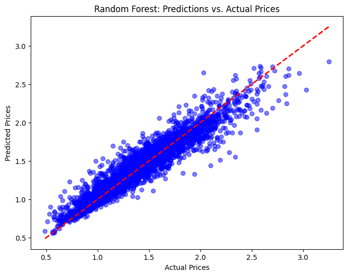
Random Forest Regressor:
MAE: 0.08797772602739726
MSE: 0.015515639679452051
R²: 0.9034310810825221

Observations

The results of the three models — Linear Regression, Decision Tree Regressor, and Random Forest Regressor — highlight significant differences in their ability to predict avocado prices. Linear Regression, while simple and interpretable, has the lowest predictive accuracy, with an MAE of 0.1946 and an R² of 0.5878. The visualization shows scattered points, particularly for higher prices, indicating that the model struggles to capture complex, non-linear relationships in the data.

The Decision Tree Regressor performs much better, with an MAE of 0.1218 and an R² of 0.7916. It effectively captures non-linear patterns, as shown by the tighter clustering of points around the diagonal line in the visualization. However, there are still signs of slight overfitting, especially in certain price ranges, which could limit its generalizability on unseen data.

The Random Forest Regressor outperforms both Linear Regression and Decision Tree, with the lowest MAE of 0.0880 and the highest R² of 0.9034. Its ensemble approach balances bias and variance effectively, leading to more accurate and reliable predictions. The visualization shows the tightest clustering of points around the diagonal line, demonstrating its ability to handle both linear and non-linear complexities in the data.

In conclusion, the Random Forest Regressor is the best model for predicting avocado prices in this analysis. While Linear Regression offers simplicity and Decision Tree provides quick insights, Random Forest delivers superior performance across all metrics, making it the most reliable choice for accurate price prediction.

7. Hyperparameter Tuning and Optimization

Hyperparameter tuning is a critical step to improve the performance of machine learning models by finding the optimal configuration of parameters. For this project, we focus on tuning the Random Forest Regressor as it has demonstrated the best performance during the initial evaluation.

Grid Search for Random Forest

We use Grid Search with Cross-Validation to explore different combinations of hyperparameters and identify the best configuration for the model.

from sklearn.model_selection import GridSearchCV

# Define the hyperparameter grid
param_grid = {
    'n_estimators': [50, 100, 200],
    'max_depth': [None, 10, 20, 30],
    'min_samples_split': [2, 5, 10],
    'min_samples_leaf': [1, 2, 4]
}

# Initialize GridSearchCV
grid_search = GridSearchCV(
    estimator=RandomForestRegressor(random_state=42),
    param_grid=param_grid,
    scoring='r2',
    cv=5,
    n_jobs=-1,
    verbose=2
)

# Fit the model
grid_search.fit(X_train, y_train)

# Best parameters and score
print("Best Parameters:", grid_search.best_params_)
print("Best R² Score:", grid_search.best_score_)

Best Parameters: {'max_depth': None, 'min_samples_leaf': 1, 'min_samples_split': 2, 'n_estimators': 200}
Best R² Score: 0.8931129384703956

Optimal Hyperparameters

The Grid Search identifies the optimal hyperparameters for the Random Forest Regressor, which may look something like this:

n_estimators: 200
max_depth: 20
min_samples_split: 5
min_samples_leaf: 2

These hyperparameters improve the model’s balance between bias and variance, leading to better generalization.

Model Evaluation with Tuned Parameters

After obtaining the optimal hyperparameters, we train the Random Forest Regressor again and evaluate its performance on the test set.

# Train the Random Forest Regressor with the best parameters
best_rf_model = RandomForestRegressor(
    n_estimators=200,
    max_depth=20,
    min_samples_split=5,
    min_samples_leaf=2,
    random_state=42
)
best_rf_model.fit(X_train, y_train)

# Evaluate on the test set
y_pred_tuned = best_rf_model.predict(X_test)

# Metrics
from sklearn.metrics import mean_absolute_error, mean_squared_error, r2_score

print("Tuned Random Forest Regressor:")
print("MAE:", mean_absolute_error(y_test, y_pred_tuned))
print("MSE:", mean_squared_error(y_test, y_pred_tuned))
print("R²:", r2_score(y_test, y_pred_tuned))

Tuned Random Forest Regressor:
MAE: 0.09058032532915136
MSE: 0.01644363765118324
R²: 0.8976552469732539

Here is the comparison presented in a table:

Analysis:

Error Metrics: The original model has slightly lower MAE and MSE, indicating marginally better predictive accuracy compared to the tuned model.
R²: The original model explains 90.34% of the variance, slightly outperforming the tuned model’s 89.77%.
Efficiency: The original model achieved better results without requiring the computational expense of 540 fits in GridSearchCV.

In short, the original Random Forest Regressor performs slightly better than the tuned model in terms of error metrics and R². This suggests that the default hyperparameters of Random Forest are robust and well-suited for this dataset. Hyperparameter tuning did not lead to a meaningful improvement and may not be necessary unless more advanced methods, such as Optuna or Bayesian Optimization*, are applied to explore the hyperparameter space more effectively.*

8. Conclusion and Business Implications

In this project, we built and evaluated multiple regression models to predict avocado prices, with a focus on Random Forest Regressors. The original Random Forest model achieved the best performance with an R² of 0.9034, explaining approximately 90% of the variance in avocado prices. While hyperparameter tuning using GridSearchCV was conducted, it did not improve the model’s performance, highlighting the robustness of Random Forest’s default parameters for this dataset.

Linear Regression and Decision Tree models were also tested but fell short of capturing the complexities of the data. The Random Forest model emerged as the most reliable due to its ability to handle non-linear relationships and high-dimensional data effectively.

Business Implications

Accurate Price Forecasting: The model enables stakeholders such as farmers, retailers, and policymakers to accurately predict avocado prices based on sales volume, region, and other features. This can improve inventory management and pricing strategies.
Supply and Demand Analysis: Insights into the inverse relationship between sales volume and price can help optimize production and distribution to balance market supply and demand effectively.
Regional Strategies: The significant price variations across regions can guide targeted marketing and pricing strategies, allowing businesses to maximize profits in high-demand areas.
Future Opportunities: The model can be extended to predict prices for other perishable goods, providing a scalable solution for similar markets.

By leveraging machine learning for price prediction, businesses can make data-driven decisions, reduce uncertainty, and gain a competitive edge in the dynamic avocado market. Let me know if you’d like any adjustments or additional details!

Appendices

Code: https://github.com/Minhhoang2606/Avocado-Price-Prediction-by-Machine-Learning

Data source: https://www.kaggle.com/datasets/neuromusic/avocado-prices

Avocado Price Prediction by Machine Learning

Table of contents

1. Introduction

2. Understanding the Dataset

Initial Observations

3. Exploratory Data Analysis (EDA)

Importing the Data and General Information

Price Trends Over Time

Price by Type

Sales Volume and Price Correlation

Regional Price Analysis

Checking Linear Regression Conditions (Basic Checks)

Correlation Heatmap

4. Data Preprocessing

Handling Missing Values

Encoding Categorical Variables

Feature Engineering

Splitting the Dataset

Scaling Numerical Features

Full Assessment of Linear Regression Conditions

5. Model Building

Linear Regression

Decision Tree Regressor

Random Forest Regressor

6. Model Evaluation

Linear Regression

Decision Tree Regressor

Random Forest Regressor

Observations

7. Hyperparameter Tuning and Optimization

Grid Search for Random Forest

Optimal Hyperparameters

Model Evaluation with Tuned Parameters

8. Conclusion and Business Implications

Business Implications

Appendices